Results matching “Weekly challenge”

To compute a constant of calculus
(A treatise on multiple ways)

𝑒 is for economics

The first task of the 21st Weekly Challenge was a very old one:
to find (what would eventually become known as) Euler’s number.

The story starts back in 1683 with Jacob Bernoulli, and his investigation of the mathematics of loan sharking. For example, suppose you offered a one-year loan of $1000 at 100% interest, payable annually. Obviously, at the end of the year the markclient has to pay you back the $1000, plus ($1000 × 100%) in interest...so you now have $2000. What can I say? It’s a sweet racket!

But then you get to thinking: what if the interest got charged every six months? In that case, after six months they already owe you $500 in interest ($1000 x 100% × 612), on which amount you can immediately start charging interest as well! So after the final six months they now owe you the original $1000 plus the first six months interest, plus the second six months interest, plus the second six months interest on the first six months interest: $1000 + ($1000 × 50%) + ($1000 × 50%) + ($1000 × 50% × 50%). Which is $2250.
Which is an even sweeter racket.

Of course it’s easier to calculate what they owe you mathematically: $1000 × (1 + ½)2
The added ½ comes from charging half the yearly interest every six months.
The power of 2 comes from charging that interest twice a year.

But why stop there? Why not charge the interest monthly instead? Then you get back the original $1000, plus $83.33 interest (i.e. 112 of $1000) for the first month, plus $90.28 interest for the second month (i.e. 112 of: $1000 + $83.33), plus $97.80 interest for the third month (i.e. 112 of: $1000 + $83.33 + $90.28), et cetera. In other words: $1000 x (1 + 112)12
or $2613.04. Nice.

If we charged interest daily, we’d get back $2714.57 (i.e. $1000 x (1 + 1365)365).
If we charged it hourly, we’d get back $2718 (i.e. $1000 x (1 + 18760)8760).
If we charged by the minute, we’d get back $2718.27 (i.e. $1000 x (1 + 1525600)525600).

Bernoulli then asked the obvious question: what’s the absolute most you could squeeze outa deese pidgeons? Just how much would you get back if you charged interest continuously?
In other words, what is the multiplier on your initial $1000 if you charge and accumulate interest at every instant? Or, mathematically speaking, what is the limit as x→∞ of (1 + 1x)x?

The answer to that question is the transcendental numeric constant 𝑒:

    2.7182818284590452353602874713526624977572470936999595749669...

Which is named after Leonhard Euler instead of Jacob Bernoulli because
(a) Euler was the first person to use it explicitly in a published scientific paper, and
(b) it really does make everything so much simpler if we just name everything after Euler.


𝑒 is for elapsed

So, given that 𝑒 is the limit of (1 + 1x)x, for increasingly large values of x, we could compute progressively more accurate approximations of the constant with just:

    for 1, 2, 4 ... ∞ -> \x {
        say (1 + x⁻¹) ** x
    }

...which produces:

    2
    2.25
    2.441406
    2.565784514
    2.6379284973666
    2.676990129378183
    2.697344952565099
    2.7077390196880207
    2.7129916242534344
    2.7156320001689913
    2.7169557294664357
    2.7176184823368796
    2.7179500811896657
    2.718115936265797
    2.7181988777219708
    2.718240351930294
    2.7182610899046034
    2.7182714591093062
    2.718276643766046
    2.718279236108013
    ⋮

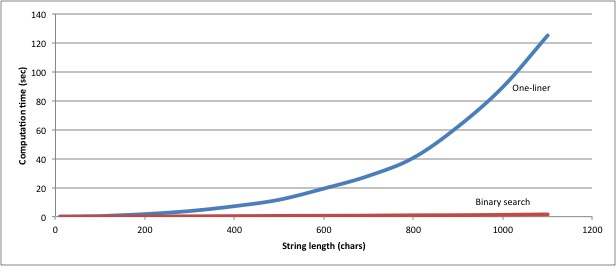
That’s an easy solution, but not a great one. After 20 iterations, at N=524288, it’s still only accurate to five decimal places (2.718279236108013).

More importantly, it’s a slow solution. How slow?
Let’s whip up an integrated timing mechanism to tell us:

    # Evaluate the block and add timing info to the result...
    sub prefix:<timed> (Code $block --> Any) {
        # Represent added timing info...
        role Timed {
            # Store the actual timing...
            has Duration $.timing;

            # When stringified, append the timing...
            my constant FORMAT = "%-20s  [%.3f𝑠]";
            method Str  { sprintf FORMAT, callsame, $.timing }
            method gist { self.Str }
        }

        # Evaluate the block, mixing timing info into result...
        return $block() but Timed(now - ENTER now);
    }

Here we create a new high-precedence prefix operator: timed. It’s an genuine operator, even though its symbol is also a proper identifier. We could just as easily have named it with an ASCII or Unicode symbol if we’d wanted to:

# Vaguely like a clock face...
sub prefix:« (<) » (Code $block --> Any) {…}

# Exactly like a stopwatch...
sub prefix:« ⏱ » (Code $block --> Any) {…}

Even without the fancy symbols, we still want an operator rather than a subroutine because
the precedence of a regular subroutine call is too low. If timed had been declared as
sub timed we wouldn’t be able to place a timed block in a surrounding argument list,
as the call to timed would attempt to gobble up all the following arguments, and then discover it is only allowed one:

say timed { expensive-func() }, " finished at ", now;
# Too many positionals passed; expected 1 argument but got 3
# in sub timed at demo.p6 line 5

Making timed a prefix operator allows the compiler to know that it can only ever take a single argument, so inline calls like the one above work fine.

Note that, as we’re feeling in need of a little extra discipline today, we’re going to make use of Raku’s type system and strictly type every variable and parameter we use. Of course, because Raku’s static typing is gradual, the code would still work exactly the same if we later removed every one of these type declarations...except then the compiler would not be able to protect us quite so well from our own stupidity.

The timed operator takes a Code object as its argument, executes it ($block()), augments the result with extra timing information, and returns the augmented result,
which can be of any type (--> Any).

That timing information is added to the block’s result by mixing into the returned object some extra capabilities defined by a generic class component (a role) named Timed.
The role confers the ability to store and access a duration (has Duration $.timing), as well as methods for enhancing how a timed object is stringified and printed (method Str and method gist). The overridden .Str method calls the object's original version
of the same method (callsame) to do the actual work, then appends the timing information
to it, neatly formatted in a sprintf. The overridden .gist just reuses .Str.

The most interesting feature is that, when we add the timing information to the result of the block (but Timed(...)), we calculate the duration of the block’s execution by subtracting the instant after the block executes (now) from the current instant when the surrounding subroutine was entered (ENTER now). Prefixing any expression with ENTER sets up a “phaser” (yeah, we know: we’re incurable geeks). A phaser is a block or thunk that executes when the surrounding block is entered. The ENTER then remembers the value generated by the thunk, and evaluates to it when the surrounding code executes: in this case, when it tries to subtract the value of the ENTER from the value of now.

You can use this same technique anywhere in Raku, as a handy way to time any particular block of code. You can also use other phasers (such as LEAVE, which executes when control leaves the surrounding block) to inline the entire operation into an easily pasteable snippet. For example, to time each iteration of a for loop, you could add a single line to the start of the loop block:

for @values -> $value {
LEAVE say "$value took ", (now - ENTER now), " seconds";

do-something-expensive-with($value);
do-something-else-protracted-with($value);
do-the-last-costly-thing-with($value);
}

So now we can easily time any block of code, simply by prefixing the block with the timed operator. And when we do that in our calculation loop:

    for 1, 2, 4 ... ∞ -> \x {
        say timed { (1 + x⁻¹) ** x }
    }

...we find that we’re going to be waiting an exponentially long time for better accuracy:

    ⋮
    2.7176184823368796    [0.001𝑠]
    2.7179500811896657    [0.002𝑠]
    2.718115936265797     [0.011𝑠]
    2.7181988777219708    [0.051𝑠]
    2.718240351930294     [0.241𝑠]
    2.7182610899046034    [1.123𝑠]
    2.7182714591093062    [4.802𝑠]
    2.718276643766046     [21.468𝑠]
    2.718279236108013     [106.543𝑠]
    ⋮

Clearly, we need a much better algorithm.


𝑒 is for extrema

In 100 Great Problems of Elementary Mathematics Heinrich Dörrie shows that, just as (1+1x)x is the lower bound on 𝑒 as x → ∞, so (1 + 1x)x+1 is the upper bound. So we can get a much better approximation of 𝑒 for the same value of N by taking the average of those two bounding values:

    for 1, 2, 4 ... ∞ -> \x {
        say timed {
            ½ × sum (1 + x⁻¹)**(x),
                    (1 + x⁻¹)**(x+1)
        }
    }

which produces:

    3                     [0.001𝑠]
    2.8125                [0.000𝑠]
    2.746582              [0.000𝑠]
    2.72614604607         [0.000𝑠]
    2.7203637629093063    [0.000𝑠]
    2.7188181001497167    [0.001𝑠]
    2.718417960007014     [0.001𝑠]
    2.718316125233677     [0.000𝑠]
    2.7182904360195543    [0.000𝑠]
    2.718283984544156     [0.000𝑠]
    2.7182823680062143    [0.000𝑠]
    2.718281963411669     [0.001𝑠]
    2.718281862205436     [0.005𝑠]
    2.7182818368966726    [0.021𝑠]
    2.718281830568581     [0.101𝑠]
    2.718281828986445     [0.456𝑠]
    2.7182818285908974    [2.171𝑠]
    2.7182818284920085    [9.628𝑠]
    2.718281828467286     [46.717𝑠]
    2.718281828461105     [206.456𝑠]
    ⋮

That’s ten correct decimal digits (2.7182818284920085) before it hits the exponential wall. Better, but still not nearly good enough.


𝑒 is for evaluation

It looks like we’re going to need to try a lot of different techniques, over a wide range of values. So it would be handy to have a simpler way of specifying a series of tests like these,
and a better way of seeing how well or poorly they perform.

So we’re going to create a framework that will let us test various techniques more simply, like so:

    #| Bernoulli's limit
    assess -> \x { (1 + x⁻¹)**(x) }

    #| Dörrie's bounds
    assess -> \x {
        ½ × sum (1 + x⁻¹)**(x),
                (1 + x⁻¹)**(x+1)
    }

Or, if we prefer, to specify a more appropriate range of trial values than just 1..∞, like so:

#| Dörrie's bounds
assess -> \x=(1,10,100...10⁶) {
½ × sum (1 + x⁻¹)**(x),
(1 + x⁻¹)**(x+1)
}

Either way, the assess function will calculate each result, determine when to give up on slow computations, tabulate the outcomes, colour-code their accuracy, and print them out neatly labelled, like so:

[1] Bernoulli's limit (x = 1): 2 [0.001𝑠] (x = 2): 2.25 [0.000𝑠] (x = 4): 2.441406 [0.000𝑠] (x = 8): 2.565784514 [0.000𝑠] (x = 16): 2.6379284973666 [0.000𝑠] (x = 32): 2.676990129378183 [0.000𝑠] (x = 64): 2.697344952565099 [0.000𝑠] (x = 128): 2.7077390196880207 [0.000𝑠] (x = 256): 2.7129916242534344 [0.000𝑠] (x = 512): 2.7156320001689913 [0.000𝑠] (x = 1024): 2.7169557294664357 [0.000𝑠] (x = 2048): 2.7176184823368796 [0.001𝑠] (x = 4096): 2.7179500811896657 [0.003𝑠] (x = 8192): 2.718115936265797 [0.011𝑠] (x = 16384): 2.7181988777219708 [0.052𝑠] (x = 32768): 2.718240351930294 [0.250𝑠] (x = 65536): 2.7182610899046034 [1.175𝑠] (x = 131072): 2.7182714591093062 [5.337𝑠]

[4] Dörrie's bounds (x = 1): 3 [0.001𝑠] (x = 2): 2.8125 [0.000𝑠] (x = 4): 2.746582 [0.000𝑠] (x = 8): 2.72614604607 [0.000𝑠] (x = 16): 2.7203637629093063 [0.000𝑠] (x = 32): 2.7188181001497167 [0.000𝑠] (x = 64): 2.718417960007014 [0.001𝑠] (x = 128): 2.718316125233677 [0.001𝑠] (x = 256): 2.7182904360195543 [0.000𝑠] (x = 512): 2.718283984544156 [0.000𝑠] (x = 1024): 2.7182823680062143 [0.000𝑠] (x = 2048): 2.718281963411669 [0.001𝑠] (x = 4096): 2.718281862205436 [0.004𝑠] (x = 8192): 2.7182818368966726 [0.025𝑠] (x = 16384): 2.718281830568581 [0.109𝑠] (x = 32768): 2.718281828986445 [0.500𝑠] (x = 65536): 2.7182818285908974 [2.369𝑠] (x = 131072): 2.7182818284920085 [10.474𝑠]

To implement all that, we start with a generic class component (i.e. another role)
suitable for storing, vetting, and formatting whatever the data we’re collecting:

    # Define a new type: Code that takes exactly one parameter...
    subset Unary of Code where *.signature.params == 1;

    # Reportable values, assessed against a target...
    role Reportable [Cool :$target = ""]
    {
        # Track reportable objects and eventually display them...
        state Reportable @reports;
        END @reports».display: @reports».width.max;

        # Add reportable objects to tracking list, and validate...
        submethod TWEAK (Unary :$check = {True}) {
            @reports.push: self;
            $check(self);
        }

        # Each report has a description and value...
        has Str  $.desc  handles width => 'chars';
        has Cool $.value handles *;

        # Display the report in two columns...
        method display (Int $width) {
            printf "%*s: %s\n", $width, $!desc, &.assess-value;
        }

        # Colour-code the value for display...
        method assess-value () {
            # Find leading characters that match the target...
            my Int $correct
                = ($!value ~^ $target).match( /^ \0+/ ).chars;

            # Split the value accordingly...
            $!value.gist ~~ /^ $<good> = (. ** {$correct})
                               $<bad>  = (\S*)
                               $<etc>  = (.*)
                            /;

            # Correct chars: blue; incorrect chars: red...
            use Terminal::ANSIColor;
            return colored($<good>.Str, 'blue')
                 ~ colored($<bad>.Str,  'red')
                 ~ $<etc>
        }
    }

We start by creating a new subtype (subset Unary) of the built-in Code type (i.e. the general type of blocks, lambdas, subroutines, etc.) This new subtype requires that the
Code object must take exactly one argument (where *.signature.params == 1).
Because (almost) everything in Raku is an object, it’s easy for the language to provide
these types of detailed introspection methods on values, variables, types, and code.

Next we create a pluggable component (role Reportable) for building classes that generate self-organizing reports. This role is parameterized to take a named value (:$target) that will subsequently be used to assess the accuracy of individual values being reported. That target value is specified to be of type Cool, which allows it to be a string, a number, a boolean, a duration, a hash, a list, or any other type automatically convertible to a string or number. This type constraint will ensure that any value reported will later be able to be assessed correctly. The :target parameter is optional; the default target being the empty string.

The Reportable role is going to automatically track all reportable objects for us...and then generate the aggregrated report at the end of the program. So we declare a shared variable to hold each report (state Reportable @reports), with a type specifier that requires each element of the array be able to perform the Reportable role. To ensure that the reports are eventually printed, we add an END phaser:

        END @reports».display: @reports».width.max;

At the end of execution, this statement calls the .display method of each report
(@reports».display), passing it the maximum width of any report description
(@reports».width.max) so that it can format the report into two clean columns.

To accumulate these reports, we arrange for each Reportable object to automatically add itself to the shared @reports array, when it is constructed...by declaring a TWEAK submethod. A submethod is a class-specific, non-inherited method, suitable for specifying per-class initializers. The TWEAK submethod is called automatically after an object is created: usually to adjust its initial value, or to test its integrity in some way.

Here, we’re doing both: by having the submethod add each object to the report list
(@reports.push: self) and by applying any :check code passed to the constructor
($check(self)). This allows the user to pass in an arbitrary test during the constructor call and have it applied to the object once that object is initialized. We’ll see shortly how useful that can be.

Each report consists of a string description and a value that can be any Cool type, so we need per-object attributes to store them. We declare them with the has keyword and a “dot” secondary sigil to make them public:

    has Str  $.desc;
    has Cool $.value;

We also need to be able to access the string width of the description.
We could declare a method to provide that information:

    method width { $.desc.chars }

But, as this is just forwarding a request from the Reportable object to the $.desc object inside it, there’s a much easier way to achieve the same effect: we simply tell the $.desc attribute that it should handle all object-level calls to .width by calling its own .chars method. Like so:

has Str $.desc handles width => 'chars';

More significantly, we also need to be able to forward methods to the $.value attribute
(for example, to interrogate its .timing information). But as we don’t know what kind of object the value may be in each case (apart from generically being Cool), we can’t know in advance which methods we may need to forward. So we simply tell $.value to handle whatever the surrounding object itself can’t, like so:

has Cool $.value handles *;

Now we just need to implement the .display method that the END phaser will use to output each Reportable object. That method takes the width into which the description should be formatted, and prints it out justified to that width using a printf. It also prints the value, which is pre-processed using the .assess-value method.

.assess-value works out how well the value matches the target, by taking a
character-wise XOR between the two ($!value ~^ $target). For every character
(or digit in a stringified number) that matches, the XOR will produce a null character ('\0'). For every character that differs, the resulting XOR character will be something else. So we can determine how many of the initial characters of the value match the target by counting how many leading '\0' characters the XOR produces (.match( /^ \0+/ ).chars).

Then we just split the value string into three substrings using a regex, colouring the leading matches blue and the trailing mismatches red, using the Terminal::ANSIColor module.

Once we have the role available, we can build a couple of Reportable classes suited to our actual data. Each result we produce will need to be assessed against an accurate representation of 𝑒:

    class Result
        does Reportable[:target<2.71828182845904523536028747135266>]
    {}

And we’ll also want to format our report with empty lines between the various techniques we’re reporting, so we need a Reportable class whose .display method is overridden to print only empty lines:

    class Spacer
        does Reportable
    {
        method display (Int) { say "" }
    }

Finally we build the assess subroutine itself:

    constant TIMEOUT = 3;  # seconds;

    # Evaluate a block over a range of inputs, and report...
    sub assess (Unary $block --> Any) {
        # Introspect the block's single parameter...
        my Parameter $param    = $block.signature.params[0];
        my Bool      $is-topic = $param.name eq '$_';

        # Extract and normalize the range of test values...
        my Any @values = do given try $param.default.() {
            when !.defined && $is-topic { Empty           }
            when !.defined              {    1, *×2 ... ∞ }
            when .?infinite             { .min, *×2 ... ∞ }
            default                     { .Seq            }
        }

        # Introspect the test description (from doc comments)...
        my Str $label = "[$block.line()] {$block.WHY // ''}".trim;

        # New paragraph in the report...
        Spacer.new;

        # Run all tests...
        for @values Z $label,"",* -> ($value, $label) {
            Result.new:
                desc  => "$label ($param.name() = $value)",
                value => timed { $block($value) },
                check => { last if .timing > TIMEOUT }
        }
        if !@values {
            Result.new:
                desc  => $label,
                value => timed { $block(Empty) }
        }
    }

The subroutine takes a single argument: a Code object that itself takes a single parameter (which we enforce by giving the parameter the type Unary).

We immediately introspect that one parameter ($block.signature.params[0]),
which is (naturally) a Parameter object, and store it in a suitably typed variable
(my Parameter $param). We also need to know whether the parameter is the
implicit topic variable (a.k.a. $_), so we test for that too.

Once we have the parameter, we need to determine whether the caller gave it a default value...which will represent the set of values for which we are to assess the code in the block passed to assess. In other words, if the user writes:

assess -> \N=1..100 { some-function-of(N) }

...then we need to extract the default value (1..100) so we can iterate through those values and pass each in turn into the block.

We can extract the parameter’s default value (if any!) by calling the appropriate introspection method: $param.default, which will return another Code object that produces the default value when called. Hence, to get the actual default value we need to call .default, then call the code .default returns. That is: $param.default.()

Of course, the parameter may not have a default value, in which case .default will return an undefined value. Attempting the second call on that undefined value would be fatal, so we make the attempt inside a try, which converts the exception into yet another undefined value.

We then test the extracted default value to determine what it means:

    when !.defined && $is-topic { Empty           }
    when !.defined              {    1, *×2 ... ∞ }
    when .?infinite             { .min, *×2 ... ∞ }
    default                     { .Seq            }

If it’s undefined, then no default was specified, so we either use an empty list as our test values (if the parameter is just the implicit topic, in which case it’s a parameterless one-off trial), or else we use the endlessly doubling sequence 1, 2, 4 ... ∞. Using this sequence instead of 1..∞ gives us reasonable coverage at every numeric order of magnitude, without the tedium of trying every single possible value.

If the default was a range to infinity (when .?infinite), then we adjust it to similar sequence of doubling values to infinity, starting at the same lower bound (.min). And if the value is anything else, we just use it as-is, only converting it to a sequence (.Seq).

Once we have the test values, we need a description for the overall test. We could have simply added a second parameter to assess, but the powerful introspective capabilities of Raku offer a more interesting alternative...

We need to convey three pieces of information: the line number at which the call to assess was made, a description of the trial being assessed, and the trial value for each trial. However, to avoid uncomely redundancy, only the first trial needs to be labelled with the line number and description; subsequent trials need only show the next trial value.

We can get the line number by introspecting the code block: $block.line()
But where can we get the description from?

Well...why not just read it directly from the comments?!

In Raku, any comment that starts with a vertical bar (i.e. #| Your comment here) is a special form of documentation known as a declarator block. When you specify such a comment, its contents are automatically attached to the first declaration following the comment. That might be a variable declared with a my, a subroutine declared with a sub or multi, or (in this case) an anonymous block of code declared between two braces.

In other words, when we write:

    #| Bernoulli's limit
    assess -> \x { (1 + x⁻¹)**(x) }

...the string "Bernoulli's limit" is automatically attached to the block that is passed into assess. We could also put the documentation comment after the block, by using #= as the comment introducer, instead of #|:

    assess -> \x { (1+x⁻¹)**x }   #= Bernoulli's limit

Either way, Raku’s advanced introspective facilities mean that we can retrieve that
documentation during program execution, simply by calling the block’s .WHY method
(because comments are supposed to tell you “WHY”, not “HOW”).

So we can generate our description by asking the block for its line number and its documentation, making do with an empty string if no documentation comment was supplied ("[$block.line()] {$block.WHY // ''}").

Now we’re ready to run our tests and generate the report. We start by inserting an empty line into the report...by declaring a Spacer object. Then we iterate through the list of values, and their associated labels, interleaving the two with a “zip” operator (Z). The labels are the initial label we built earlier, then an empty string, then a “whatever” (*), which tells the zip operator to reuse the preceding empty string as many times as necessary to match the remaining elements of @values. That way, we get the full label on the first line of the trial, but no repeats of it thereafter.

The zip produces a series of two-element arrays: one value, one label. We then iterate through these, building an appropriate Result object for each test:

    Result.new:
        desc  => "$label ($param.name() = $value)",
        value => timed { $block($value) },
        check => { last if .timing > TIMEOUT }

The description for the report is the label, followed by the block’s parameter name ($param.name()) and the current trial value being passed to it on this iteration ($value). The value for the report is just the timed result of calling the block with the current trial value passed to it (timed { $block($value) }).

But we also want to stop testing when the tests get too slow, so we pass the Result constructor a check argument as well, which causes its TWEAK submethod to execute the check block once the result has been added to the report list. Then we arrange for the check block to terminate the surrounding for loop (i.e.last) if the timing of the new object exceeds our chosen timeout. The call to .timing will be invoked on the Result object, which (not having a timing method itself) will delegate the call to its $.value attribute, which we specified to handle “whatever” methods the object itself can’t deal with.

The only thing left to do is to cover the edge-case where the user provides no test values
at all (i.e. when there are no @values to iterate through). That can happen either when an explicit empty list of default values is passed to assert, or when the block passed in doesn’t explicitly declare a parameter at all (and therefore defaults to the implicit topic parameter: $_). In either case, we need to call the block exactly once, without any argument. So if the array of test values has no elements (if @values.elems == 0),
we instantiate a single Result object, passing it the full label, and the timed result of calling the block with a (literally) empty argument list:

        if !@values {
            Result.new:
                desc  => $label,
                value => timed { $block(Empty) }
        }

And we’re done. We now have an introspective and compact way of performing multiple trials on a block, across a range of suitable values, either explicit or inferred, with automatic timing of—and timeouts on—each trial.

So let’s get back to computing the value of 𝑒...


𝑒 is for eversion

The constant 𝑒 is associated with Jacob Bernoulli in another, entirely unrelated way. In his posthumous 1712 publication, Ars Conjectandi, Bernoulli explored the mathematics of binomial trials: random experiments in which the results are strictly binary: success or failure, true or false, yes or no, heads or tails.

One of the results of binomial theory has to do with the probability of extremely bad luck.
If we conduct a random binomial trial where the probability of success is 1k, then the probability of failure must be 1 - 1k. Which means that, if we repeat our same random trial
k times, then the probability of failing every time is (1 - 1k)k. As k grows larger, this probability increases from zero (for k=1), to 0.25 (for k=2), to 0.296296296296... (for k=3), to 0.31640625 (for k=4), gradually converging on an asymptotic value of 0.36787944117144233... (for k=∞). And the value 0.36787944117144233... is exactly 1𝑒.

Which means that (1 - 1k)-k must tend towards 𝑒 as k tends to ∞. So we can try:

    #| Bernoulli trials
    assess -> \k=2..∞  { (1 - k⁻¹) ** -k }

...which tells us:

[20] Bernoulli trials (k = 2): 4 [0.000𝑠] (k = 4): 3.160494 [0.000𝑠] (k = 8): 2.910285368 [0.000𝑠] (k = 16): 2.808403965576447 [0.000𝑠] (k = 32): 2.762009089976452 [0.000𝑠] (k = 64): 2.7398271814872146 [0.000𝑠] (k = 128): 2.7289767306942787 [0.000𝑠] (k = 256): 2.7236100544173554 [0.000𝑠] (k = 512): 2.720941162086445 [0.000𝑠] (k = 1024): 2.7196103037796897 [0.000𝑠] (k = 2048): 2.7189457686628256 [0.001𝑠] (k = 4096): 2.7186137242488035 [0.002𝑠] (k = 8192): 2.7184477577823865 [0.011𝑠] (k = 16384): 2.718364788478643 [0.059𝑠] (k = 32768): 2.7183233073084274 [0.265𝑠] (k = 65536): 2.718302567593645 [1.232𝑠] (k = 131072): 2.7182921979538235 [6.135𝑠]

Which, sadly, converges no faster than Bernoulli’s original loan sharking scheme.


𝑒 is for exclamation

Despite its disappointing performance, the Bernoulli trials approach highlights a useful idea. The constant 𝑒 appears in a great many other mathematical equations, all of which we could rearrange to produce a formula starting: 𝑒 = ...

For example, in 1733 Abraham de Moivre first published an asymptotic approximation for the factorial function, which (just a few days later!) was refined by James Stirling, after whom the approximation is now named. That approximation is: n! n × (n𝑒)n
with the approximation becoming more accurate as n becomes larger.

Rearranging that equation, we get: 𝑒 n/nn!

For which we’re going to need both an n-th root operator and a factorial operator. Both of which are missing from standard Raku. Both of which are trivially easy to add to it:

    # n-th root of x...
    sub infix:<√> (Int $n, Int $x --> Numeric) is tighter( &[**] ) {
        $x ** $n⁻¹
    }

    # Factorial of x...
    sub postfix:<!> (Int $x --> Int)  {
        [×] 1..$x
    }

The new infix operator is specified to have a precedence just higher than the existing ** exponentiation operator (is tighter( &[**] )). It simply raises the value after the to the reciprocal of the value before the .

The new postfix ! operator multiplies together all the numbers less than or equal to its single argument (1..$x), using a reduction by multiplication ([×]).

With those two new operators available, we can now write:

    #| de Moivre/Stirling approximation
    assess -> \n { n / n√n! }

Unfortunately, the results are less than satisfactory:

[30] de Moivre/Stirling approximation (n = 1): 1 [0.000𝑠] (n = 2): 1.414213562373095 [0.000𝑠] (n = 4): 1.80720400721969 [0.000𝑠] (n = 8): 2.1252005594420327 [0.000𝑠] (n = 16): 2.352779665665871 [0.000𝑠] (n = 32): 2.501898064970579 [0.000𝑠] (n = 64): 2.5938155227045367 [0.001𝑠] (n = 128): 2.6481531254600723 [0.001𝑠] (n = 256): 0 [0.001𝑠] (n = 512): 0 [0.006𝑠] (n = 1024): 0 [0.011𝑠]

This approach converges on 𝑒 even slower than the previous ones, and for the first time
Raku has actually failed us when it comes to a numerical calculation. Those zeroes are indicating that the compiler has been unable to take the 256th root of the factorial of 256.
Or deeper roots of higher numbers.

It computed the factorial itself (i.e. 8578177753428426541190822716812326251577815202 79485619859655650377269452553147589377440291360451408450375885342336584306 15719683469369647532228928849742602567963733256336878644267520762679456018 79688679715211433077020775266464514647091873261008328763257028189807736717 81454170250523018608495319068138257481070252817559459476987034665712738139 28620523475680821886070120361108315209350194743710910172696826286160626366 24350228409441914084246159360000000000000000000000000000000000000000000000 00000000000000000) without difficulty, but then taking the 256th root of that huge number (by raising it to the power of 1256) failed. It incorrectly produced the value ∞, whereupon n divided by that wrong result produced the zero. The point of failure seems to be around 170! or 10308, which looks suspiciously like an internal 64-bit floating-point representation limit.

Of course, we could work around that limitation, by changing the way we compute n-th roots. For example, the n-th root of a number also given by: 10log10Xn

So we could try:

# n-th root of x...
sub infix:<√> (Int $n, Int $x --> Numeric) is tighter(&[**]) {
10 ** (log10($x) / $n)
}

...but we get exactly the same problem: the built-in log10 function breaks at around 10308, meaning we can’t apply it to factorials of numbers greater than 170.

But when X is an integer, there’s a surprisingly good approximation to log10X that doesn’t have this 10308 limitation at all: we simply count the number of digits in X and subtract ½.
In the worst cases, this result is out by no more than ±0.5, but that means its average error over a sufficiently large range of values...is zero.

Using that approximation for n-th roots:

# n-th root of x...
sub infix:<√> (Int $n, Int $x --> Numeric) is tighter(&[**]) {
10 ** (($x.chars - ½) / $n)
}

...we can now extend our assessment of the de Moivre/Stirling approximation far beyond n=170. In which case we find:

[30] de Moivre/Stirling approximation (n = 1): 0.31622776601683794 [0.000𝑠] (n = 2): 1.1246826503806981 [0.000𝑠] (n = 4): 1.6867860137143293 [0.000𝑠] (n = 8): 2.190735707411489 [0.000𝑠] (n = 16): 2.2928201123791405 [0.000𝑠] (n = 32): 2.4875680967640825 [0.000𝑠] (n = 64): 2.5570691577279274 [0.001𝑠] (n = 128): 2.6522607579574027 [0.001𝑠] (n = 256): 2.6898269484112647 [0.005𝑠] (n = 512): 2.69742667825642 [0.006𝑠] (n = 1024): 2.7080909004243128 [0.012𝑠] (n = 2048): 2.711166091674111 [0.040𝑠] (n = 4096): 2.7150077947508775 [0.159𝑠] (n = 8192): 2.716181527473568 [0.678𝑠] (n = 16384): 2.7171648275814224 [3.049𝑠]

To our disgust, the convergence of this approach clearly does not accelerate at higher values of n.

In fact, even when n is over a million, the result is still only accurate to three decimal places; worse even than the classic palindromic fractional approximation:

    #| Palindromic fraction
    assess {   878
             / 323
           }

...which gives us:

[40] Palindromic fraction: 2.718266 [0.001𝑠]

Alas, the search continues.


𝑒 is for estimation

Let’s switch back to probability theory. Imagine a series of uniformly distributed random numbers in the range 0..1. For example:

    0.162532, 0.682623, 0.4052625, 0.42167261, 0.99765261, ...

If we start adding those numbers up, how many terms of the series do we need to add
together before the total is greater than 1? In the above example, we’d need to add
the first three values to exceed 1. But in other random sequences we’d need to add only
two terms (e.g. 0.76217621, 0.55326178, ...) and occasionally we’d need to add quite a few more (e.g. 0.1282827, 0.00262671, 0.39838722, 0.386272617, 0.77282873, ...). Over a large number of trials, however, the average number of random values required for the sum to exceed 1 is (you guessed it): 𝑒.

So, if we had a source of uniform random values in the range 0..1, we could get an approximate value for 𝑒 by repeatedly adding sufficient random values to exceed 1,
and then averaging the number of values we required each time, over multiple trials.
Which looks like this in Raku:

    #| Stochastic approximation
    assess -> \trials=(10², 10³, 10⁴, 10⁵, 10⁶) {
        sum( (1..trials).map:
                { ([\+] rand xx ∞).first(* > 1):k + 1 }
        )
        / trials
    }

That is: we conduct a specified number of trials (1..trials), and for each trial (.map:)
we generate an infinite number of uniform random values (rand xx ∞), which we then convert to a list of progressive partial sums ([\+]). We then look for the first of these partial sums that exceeds 1 (.first(* > 1)), find out its index in the list (:k) and add 1
(because indices start from zero, but counts start from 1).

The result is a list of counts of how many random values were required to exceed one in each of our trials. As 𝑒 is the average of those counts, we sum them and divide by the number of trials. And find:

[50] Stochastic approximation (trials = 100): 2.62 [0.020𝑠] (trials = 1000): 2.7 [0.045𝑠] (trials = 10000): 2.7179 [0.357𝑠] (trials = 100000): 2.7256 [3.651𝑠] (trials = 1000000): 2.718698 [43.185𝑠]

That’s pretty good...for random guessing. If we’d kept it running for a greater number of trials, we’d eventually have gotten reasonable accuracy. But it’s unreliable: sometimes losing accuracy as the number of trials increases. And it’s slow: only three digits of accuracy after a million trials...and 40 seconds of computation. To get a useful number of correct digits we’d need billions, possibly trillions, of trials...which would require tens, or thousands, of hours of computation.

So on we go....


𝑒 is for efficiency

Or, rather, back we go. Back to 1669, to that Isaac Newton of mathematical geniuses:
Isaac Newton. In a manuscript entitled De analysi per aequationes numero terminorum infinitas Newton set out a general approach to solving equations that are infinite series,
an approach that implies a highly efficient way of determining 𝑒.

Specifically, that: 𝑒 = Σ 1k! for k from 0 to ∞

So let’s try that:

    #| Newton's series
    assess -> \k=0..∞ { sum (0..k)»!»⁻¹ }

Here we compute 𝑒 by taking increasingly longer subsets of length k from the infinite series of terms (\k=0..∞). We take the indices of the chosen terms ((0..k)), and for each
of them (») take its factorial (!). Then for each factorial (») we take its reciprocal (⁻¹).
The result is a list of the successive terms 1k!, which we finally add together (sum) to get 𝑒:

[60] Newton's series (k = 0): 1 [0.001𝑠] (k = 1): 2 [0.000𝑠] (k = 2): 2.5 [0.000𝑠] (k = 3): 2.666667 [0.000𝑠] (k = 4): 2.708333 [0.001𝑠] (k = 5): 2.716667 [0.001𝑠] (k = 6): 2.718056 [0.002𝑠] (k = 7): 2.718254 [0.001𝑠] (k = 8): 2.718279 [0.005𝑠] (k = 9): 2.718282 [0.001𝑠] (k = 10): 2.718281801 [0.001𝑠] (k = 11): 2.718281826 [0.001𝑠] (k = 12): 2.7182818283 [0.002𝑠] (k = 13): 2.718281828447 [0.002𝑠] (k = 14): 2.7182818284582 [0.002𝑠] (k = 15): 2.71828182845899 [0.002𝑠] (k = 16): 2.7182818284590423 [0.002𝑠] (k = 17): 2.718281828459045 [0.002𝑠] (k = 18): 2.718281828459045227 [0.002𝑠] (k = 19): 2.7182818284590452 [0.003𝑠] (k = 20): 2.71828182845904523534 [0.007𝑠] ⋮

Finally...some real progress. After summing only 20 terms of the infinite 1k! series, we have 19 correct decimal places, and (at last!) a reasonably accurate value of 𝑒.

And we can do even better: 𝑒 can be decomposed into many other infinite summations.
For example: in 2003 Harlan Brothers discovered that 𝑒 = Σ (2k+1)(2k)!
which we could assess with:

    #| Brothers series
    assess -> \k=0..∞ {
        sum (2 «×« (0..k) »+» 1) »/« (2 «×« (0..k))»!
    }

By making every arithmetic operator a hyperoperator, we can compute the entire series of 0..k terms in a single vector expression and then sum them to get 𝑒.

The code for the Brothers formula might be a little uglier than for Newton’s original,
but it makes up for that by converging twice as fast, giving us 19 correct decimal places from just the first ten terms in the series:

[70] Brothers series (k = 0): 1 [0.003𝑠] (k = 1): 2.5 [0.000𝑠] (k = 2): 2.708333 [0.001𝑠] (k = 3): 2.718056 [0.001𝑠] (k = 4): 2.718279 [0.001𝑠] (k = 5): 2.718281801 [0.001𝑠] (k = 6): 2.7182818283 [0.001𝑠] (k = 7): 2.7182818284582 [0.001𝑠] (k = 8): 2.7182818284590423 [0.001𝑠] (k = 9): 2.718281828459045227 [0.001𝑠] (k = 10): 2.71828182845904523534 [0.001𝑠] ⋮


𝑒 is for epsilon

We’re making solid progress on an accurate computation of 𝑒 with these two Newtonian series, but that ugly (and possibly scary) hyperoperated assessment code is still kinda irritating. And too easy to get wrong.

Given that these efficient methods all work the same way—by summing (an initial subset of) an infinite series of terms—maybe it would be better if we had a function to do that for us. And it would certainly be better if the function could work out by itself exactly how much of that initial subset of the series it actually needs to include in order to produce an accurate answer...rather than requiring us to manually comb through the results of multiple trials to discover that.

And, as so often in Raku, it’s surprisingly easy to build just what we need:

    sub Σ (Unary $block --> Numeric) {
        (0..∞).map($block).produce(&[+]).&converge
    }

We call the subroutine Σ, because that’s the usual mathematical notation for this function (okay, yes, and just because we can). We specify that it takes a one-argument block, and returns a numeric value (Unary $block --> Numeric), with the return value representing a “sufficiently accurate” summation of the series specified by the block.

To accomplish that, it first builds the infinite list of term indexes (0..∞) and passes each in turn to the block (.map($block)). It then builds successive partial sums of the resulting terms (.produce(&[+])). That is, if the block was { 1 / k! }, then the list created by the .map would be: (1, 1, 12, 16, 124, 1120, ...) and the .produce(&[+]) method call would progressively add these, producing the list: 1, 1+1, 1+1+12, 1+1+12+16, 1+1+12+16+124, 1+1+12+16+124+1120, ...)
That is: (1, 2, 2.5, 2.666, 2.708, 2.717, ...).

We set the calculation up this way because we need to be able to work out when to stop adding terms, which will be when the successive elements of the .produce list converge
to a consistent value. In other words, when two successive values differ by only an inconsequential amount.

And, conveniently, Raku has an operator that can tell us precisely that:
the is-approximately-equal-to operator (or its ASCII equivalent: =~=).

So we could write a subroutine that takes a list and returns the first “converged” value
from it, like so:

    sub converge(Iterable $list --> Numeric) {
        $list.rotor(2=>-1).first({ .head ≅ .tail }).tail
    }

The .rotor method extracts sublists of N elements from its list. Here we tell it to extract two elements at a time, but to also make them overlap, by stepping back one place (-1) between each extraction. The result is that, from a list such as (1, 2, 2.5, 2.666, 2.708, 2.717 …), we get a list of lists of every pair of adjacent values:
( (1, 2), (2, 2.5), (2.5, 2.667), (2.667, 2.708), (2.708, 2.717) …)

Then we simply step through the list of lists, looking for the first sublist in which the head and tail elements are approximately equal (.first({ .head ≅ .tail })). That gives us back a single sublist, from which we extract only the more-accurate tail element (.tail).

We can then just apply this function to the list of partial sums being produced in Σ:

(0..∞).map($block).produce(&[+]).&converge

...which is just a conveniently left-to-right way of passing the entire list into converge.
Of course, we could also have written it as a normal name-arglist style subroutine call:

converge (0..∞).map($block).produce(&[+])

...if that makes us more comfortable.

The insanely cool thing about all this—and the only reason it works at all—is that every component of the two method-call chains within Σ and converge is lazily evaluated.
Which means that .map doesn’t actually execute the block on any of the (0..∞) values, and .produce doesn’t progressively add any of them together, and .rotor doesn’t extract any overlapping pairs of them, and .first doesn’t search any of them...unless the final result requires them to. The .map only invokes the block as many times as necessary to get enough values for .produce to add, to get enough values for .rotor to extract,
to get enough values for .first to find the first approximately equal pair.

I truly love that about Raku: not only does it allow you to write code that’s concise, expressive, and elegant; your concise, expressive, elegant code is naturally efficient as well.

Meanwhile, we now have a much better (i.e. more concise, more expressive, more elegant) way of generating a highly accurate value of 𝑒:

    #| Newton's series
    assess { Σ -> \k { 1 / k! } }

    #| Brothers series
    assess { Σ -> \k { (2×k + 1) / (2×k)! } }

...which give us the straightforward answers we were looking for:

[80] Newton's series: 2.718281828459045227 [0.007𝑠]

[83] Brothers series: 2.71828182845904523534 [0.002𝑠]


𝑒 is for epigram

And that would be the end of the story...except that we’ve still ignored half of the possibilities. Every technique we’ve tried so far has been mathematical in nature.
But Raku is not just for algebraists or statisticians or probability theorists.
It’s also for linguists and authors and poets and all other lovers of natural language.

So how could we use natural language to compute an accurate value of 𝑒?

Well, it turns out that algebraists and statisticians and probability theorists have been doing that for centuries. Because once you’ve spent several hours (or days, or weeks) manually calculating the first eight digits of 𝑒, you never want to have to do that again! So you come up with a mnemonic: a sentence that helps you remember those hard-won digits.

Most mnemonics of this kind work by encoding each digit in the length of successive words.
For example, to remember the constant 1.23456789, you might encode it as:
“I am the only local Aussie abacist publicly available”. Then you just count the letters
of each word to extract the digits.

As usual, that’s trivial to implement in Raku:

    sub mnemonic(Str $text --> Str) {
        with $text.words».trans(/<punct>+/ => '')».chars {
            return "{.head}.{.tail(*-1).join}"
        }
    }

We first extract each word from the text ($text.words), and for each of them (»)
we remove any punctuation characters by translating them to empty strings
(.trans(/<punct>+/ => '')), and finally count the number of remaining
characters in each word (».chars). We then take the first element from that list of
word lengths (.head), add a dot, and then append the concatenation of the rest
of the N-1 character counts (.tail(*-1).join), and return that as the
string representation of the resulting number.

Then we test it:

    #| Mnemonic test
    assess {
        mnemonic "I am the only local Aussie abacist
                  publicly available"
    }

...which prints:

[90] Mnemonic test: 1.23456789 [0.002𝑠]

...which is clearly a very poor approximation to 𝑒.

But for three centuries people have been making up better ones.
One of the most widely used is the slightly self-deprecating:

    #| Modern mnemonic
    assess {
        mnemonic "It enables a numskull to remember
                  a sequence of numerals"
    }

...which gives us nine correct decimal places:

[100] Modern mnemonic: 2.718281828 [0.003𝑠]

If we need more accuracy, we can just compose a longer sentence. For example:

    #| Titular mnemonic
    assess {
        mnemonic "To compute a constant of calculus:
                  (A treatise on multiple ways)"
    }

...which produces one additional digit:

[110] Titular mnemonic: 2.7182818284 [0.002𝑠]

Or, for better accuracy than any of the mathematical approaches so far, we could use Zeev Barel’s self-referential description:

    #| Extended mnemonic
    assess {
        mnemonic "We present a mnemonic to memorize a constant
                  so exciting that Euler exclaimed: '!'
                  when first it was found. Yes, loudly: '!'.
                  My students perhaps will compute e, via power
                  or Taylor series, an easy summation formula.
                  Obvious, clear, elegant!"
    }

...which gives us far more accuracy than we’d ever actually need:

[120] Extended mnemonic: 2.718281828459045235360287471352662497757 [0.010s]


𝑒 is for eclectic

And even that isn’t the end of the story. Just like π (its main rival for World’s Most Awesome Mathematical Constant), 𝑒 exerts a strange fascination over the mathematically whimsical.

For example, in 1988, Dario Castellanos published the following identity: 𝑒 = 4 + π5)16
Which, translated to Raku is:

    #| Castellano's coincidence
    assess { (π⁴ + π⁵) ** ⅙ }

...and gives us seven decimal places of accuracy:

[130] Castellano's coincidence: 2.718281808611915 [0.001𝑠]

And those of us who can remember the digits 1 to 9 (or who know an Aussie abacist)
can use Richard Sabey’s formula: 𝑒 = (1 + 2-3×(4+5)).6×.7+89:

    #| Sabey's digits
    assess { (1+2**(-3×(4+5)))**(.6×.7+8⁹) }

...which (fittingly) gives us nine correct digits in total:

[140] Sabey's digits: 2.718281826838823 [0.000𝑠]

But those curiosities are as nothing compared to the true highlands of 𝑒 exploration.

For example, Maksymilian Piskorowski found that if you happen to have a spare eight 9s, you can compute 𝑒 = (99 + 9-99)999, which is accurate to a little over 369 million
decimal places.

We could translate that easily enough to Raku:

     #| Piskorowski's eight 9s
     assess { (9/9 + 9**-9**9) ** 9**9**9 }

But, alas, our assessment fails (eventually), producing a disappointing:

[150] Piskorowski's eight 9s: 1 [332242.506𝑠]

...because the value of 9-99 is so vanishingly small that adding it to 99 in Raku
merely produces 1, and then 1999 is still 1.

Piskorowski’s incalculable ⅓ billion decimal places of accuracy seemed like the (il)logical end-point of this quest. But only until the aforesaid Richard Sabey spoiled the game for everyone, by reformulating his aforementioned pan-digital formulation to: 𝑒 = (1 + 9-47×6)3285

Which is accurate to a staggering 18457734525360901453873570 decimal places
(that’s 18.4 octillion digits)...but which, tragically, immediately underflows Raku’s numeric representation when attempting to compute the initial 9-442; Raku being unable to accurately represent 1919342813113834066795298816.

Meanwhile, if you’d like to further explore these and other 𝑒-related exotica,
check out Erich Friedman’s mesmerizing Math Magic website.


𝑒 is for exquisite

There is still one higher mathematical summit for us to surmount in our quest for 𝑒.
The pinnacle of mathematical elegance, the peak of arithmetical pulchritude,
the single most beautiful equation in all of mathematics: Euler’s Identity

In 1748 Leonhard Euler published his masterwork: Introductio in analysin infinitorum,
in which he included the first mention of the general Euler Formula: 𝑒ix = cos x + i sin x.
Although not explicitly mentioned in the treatise, this formula implies a remarkable special case (at x=π) of: 𝑒 = -1 + 0i

This special-case equality is nowadays more usually written: 𝑒 + 1 = 0
Thereby uniting the five most important constants in mathematics.

Quite apart from this extraordinarily lovely unification of mathematical fundamentals,
for our purposes the significant point here is that one of the five components is 𝑒.
And, if we rearrange the formula to isolate that constant, we get: 𝑒 = (-1)1πi
which we can easily assess in Raku:

    #| From Euler's Identity
    assess { (-1) ** (π×i)⁻¹ }

Unfortunately, Raku is not (yet) smart enough to infer from the imaginary exponent that it needs to use the Complex version of the ** operator (well, yes, of course complex mathematics is already built into Raku). So we get back:

[160] From Euler's Identity: NaN [0.000𝑠]

...because the non-complex exponentiation fails when given a complex exponent,
producing the value NaN+NaN\i.

But if we start with a suitably 2D version of -1 (i.e. -1+0i), like so:

    #| From Euler's Identity
    assess { (-1+0i) ** (π×i)⁻¹ }

...we get the correct complex arithmetic, and a highly accurate answer from it:

[160] From Euler's Identity: 2.718281828459045 [0.000𝑠]


𝑒 is for effortless

It’s fitting that we have now come full circle: finding Euler’s Number
from the special case of Euler’s Formula that is Euler’s Identity.
Euler’s Ouroboros, if you will.

All that effort...to end up more or less back where we started. Which is highly appropriate,
because where we started already had the answer built in. First of all, in the form of
the standard exp function, which returns the value of 𝑒x.

So we could have tried:

    #| Built-in exp() function
    assess -> \x=1 { exp(x) }

...which would have given us:

[170] Built-in exp() function (x = 1): 2.718281828459045 [0.000𝑠]

But even that is considerably more effort that we actually need in Raku.
Because (of course) the constant itself is also built right in to the language:

    #| Built-in e constant
    assess { e }

...and produces an equally accurate result:

[180] Built-in e constant: 2.718281828459045 [0.000𝑠]

So the optimal solution to the original task was just five characters long:

    say e

...which shall henceforth be known as: “Euler’s One-liner”.

Damian

With friends like these...

C-o-rr-a-ll-i-n-g d-i-tt-o-e-d l-e-tt-e-r-s

I was going to focus this week on the first task of the 20th Weekly Challenge...but what can I say? The task was a break a string specified on the command-line into runs of identical characters:

    "toolless"        →   t  oo  ll  e  ss
    "subbookkeeper"   →   s  u  bb  oo  kk  ee  p  e  r
    "committee"       →   c  o  mm  i  tt  ee

But that’s utterly trivial in Raku:

    use v6.d;

    sub MAIN (\str) {
        .say for str.comb: /(.) $0*/
    }

And almost as easy in Perl:

use v5.30;

my $str = $ARGV[0]
// die "Usage:\n $0 <str>\n";

say $& while $str =~ /(.) \1*/gx;

In both cases, the regex simply matches any character ((.)) and then rematches exactly
the same character ($0 or \1) zero-or-more times (*). Both match operations (str.comb
and $str =~) produce a list of the matched strings, each of which we then output
(.say for... or say $& while...).

As there’s not much more to say in either case, I instead turned my attention to the second task: to locate and print the first pair of amicable numbers.


The friend of my friend is my enemy

Amicable numbers are pairs of integers, each of which has a set of proper divisors
(i.e. every smaller number by which it is evenly divisible) that happen to add up to
the other number.

For example, the number 1184 is divisible by 1, 2, 4, 8, 16, 32, 37, 74, 148, 296, and 592; and the sum of 1+2+4+8+16+32+37+74+148+296+592 is 1210. Meanwhile, the number 1210 is divisible by 1, 2, 5, 10, 11, 22, 55, 110, 121, 242, and 605; and the sum of 1+2+5+10+11+22+55+110+121+242+605 is...you guessed it...1184.

Such pairs of numbers are uncommon. There are only five among the first 10 thousand integers, only thirteen below 100 thousand, only forty-one under 1 million. And the further we go, the scarcer they become: there only 7554 such pairs less than 1 trillion. Asymptotically, their average density amongst the positive integers converges on zero.

There is no known universal formula for finding amicable numbers, though the 9th century Islamic scholar ثابت بن قره did discover a partial formula, which Euler (of course!) subsequently improved upon 900 years later.

So they’re rare, and they’re unpredictable...but they’re not especially hard to find.

In number theory, the function giving the sum of all proper divisors of N
(known as the “restricted divisor function”) is denoted by 𝑠(N):

sub 𝑠 (\N) { sum divisors(N) :proper }

That trailing :proper is an “adverbial modifier” being applied to the call to divisors(N),
telling the function to return only proper divisors (i.e. to exclude N itself from the list).
And, yeah, that’s a Unicode italic 𝑠 we’re using as the function name. Because we can.

Once we have the restricted divisor function defined, we could simply iterate through each integer i from 1 to infinity, finding 𝑠(i), then checking to see if the sum-of-divisors of that number (i.e. 𝑠(𝑠(i)) ) is identical to the original number. If we only need to find the first pair of amicable numbers, that’s just:

for 1..∞ -> \number {
my \friend = 𝑠(number);

say (number, friend) and exit
if number != friend && 𝑠(friend) == number;
}

Which outputs:

    (220, 284)

But why stop at one result? When it’s no harder to find all the amicable numbers:

for 1..∞ -> \number {
my \friend = 𝑠(number);

say (number, friend)
if number < friend && 𝑠(friend) == number;
}

Note that, because the amicable relationship between numbers is (by definition) symmetrical,
we changed the number != friend test to number < friend
...to prevent the loop from printing each pair twice:

(220, 284)
(284, 220)
(1184 1210)
(1210 1184)
(2620 2924)
(2924 2620)
(et cetera)
(cetera et)

The missing built-in

That would be the end of this story, except for one small problem: somewhat surprisingly,
Raku doesn’t have the divisors builtin we need to implement the 𝑠 function. So we’re going to have to build one ourselves. In fact, we’re going to build quite a few of them...

The divisors of a whole number are all the integers by which it can be divided leaving no remainder. This includes the number itself, and the integer 1. The “proper divisors” of a number are all of its divisors except itself. The “non-trivial divisors” of a number are all of its divisors except itself or 1. That is:

    say divisors(12);                # (1 2 3 4 5 6 12)
    say divisors(12) :proper;        # (1 2 3 4 5 6)
    say divisors(12) :non-trivial;   #   (2 3 4 5 6)

The second and third alternatives above, with the funky adverbial modifiers, are really just syntactic honey for a normal call to divisors but with an additional named argument:

    say divisors(12);                # (1 2 3 4 5 6 12)
    say divisors(12, :proper);       # (1 2 3 4 5 6)
    say divisors(12, :non-trivial);  #   (2 3 4 5 6)

In Raku it’s easiest to implement those kinds of “adverbed” functions using multiple dispatch, where each special case has a unique required named argument:

multi divisors (\N, :$proper!) { divisors(N).grep(1..^N) }
multi divisors (\N, :$non-trivial!) { divisors(N).grep(1^..^N) }

Within the body of each of these special cases of divisors, we just call the regular variant of the function (i.e. divisors(N)) and then grep out the unwanted endpoint(s).
The ..^ operator generates a range that excludes its own upper limit,
while the ^..^ operator generates a range that excludes both its bounds.
(Yes, there’s also a ^.. variant to exclude just the lower bound).

So, when the :proper option is specified, we filter the full list returned by divisors(N)
to omit the number itself (.grep(1..^N). Likewise, we exclude both extremal values when the :non-trivial option is included (.grep(1^..^N).

But what about the original unfiltered list of divisors?
How do we get that in the first place?

The naïve way to generate the full list of divisors of a number N, known as “trial division”,
is to simply to walk through all the numbers from 1 to N, keeping all those that divide N
with no remainder...which is easy to test, as Raku has the %% is-divisible-by operator:

    multi divisors (\N) {
        # Track all divisors found so far...
        my \divisors = [];

        # For every potential divisor...
        for 1..N -> \i {
            # Skip if it's not an actual divisor...
            next unless N %% i;

            # Otherwise, add it to the list...
            divisors.push: i;
        }

        # Deliver the results...
        return divisors;
    }

Except that we’re not cave dwellers and we don't need to rub sticks together like that, nor do number theory by counting on our toes. We can get the same result far more elegantly:

    multi divisors (\N) { (1..N).grep(N %% *) }

Here we simply filter the list of potential divisors (1..N), keeping only those that evenly divide N (.grep(N %% *)). The N %% * test is a shorthand for creating a Code object that takes one argument (represented by the *) and returns N %% that argument. In other words, it creates a one-argument function by pre-binding the first operand of the infix %% operator to N. If that’s a little too syntactically mellifluous for you, we could also have written it as an explicit pre-binding of the %% operator:

(1..N).grep( &infix:<%%>.assuming(N) )

...or as a lambda:

(1..N).grep( -> \i { N %% i } )

...or as an anonymous subroutine:

(1..N).grep( sub (\i) { N %% i } )

...or as a named subroutine:

my sub divisors-of-N (\i) { N %% i }

(1..N).grep( &divisors-of-N )

Raku aims to let us express ourselves in whichever notation we find most convenient, comfortable, and comprehensible.


Getting to the root of the problem

It’s hard to imagine a simpler solution to the problem of finding divisors than:

    multi divisors (\N) {  (1..N).grep(N %% *)  }

But it’s also hard to imagine a less efficient one. For example, in order to find the eight divisors of the number 2001, we have to check all 2001 potential divisors, which is 99.6% wasted effort. Even for a number like 2100—which has thirty-six divisors—we’re still throwing away over 98% of the 1..N sequence. And the bigger the number,
the smaller its relative number of divisors, and the longer it takes to find them.
There must be a better way.

And, of course, there is. The simplest improvement we can make was first published back in 1202 by Fibonacci in his magnum opus Liber Abbaci. We start by observing that the divisors of a number always come in complementary pairs; pairs that multiply together to produce the number itself. For example, the divisors of 99 are:

      1    3    9
     99   33   11

...while the divisors of 100 are:

      1    2    4    5   10
    100   50   25   20   10

...and the divisors of 101 are:

      1
    101

Notice that, in each case, the top row of divisors always contains “small” integers no greater than the square-root of the original number. And the bottom row consists entirely of N divided by the corresponding top-row divisor. So we could find half the divisors by searching the range 1..sqrt N (in just O(√N) steps), and then find the other half by subtracting each element of that list from N (also in just O(√N) steps). In Raku that look like this:

    multi divisors (\N) {
        my \small-divisors = (1..sqrt N).grep(N %% *);
        my \big-divisors   = N «div« small-divisors;

        return unique flat small-divisors, big-divisors;
    }

The div operator is integer division, and putting the double angles around it makes it
a vector operator that divides N by each element of the list of small-divisors.
The flat is needed because the two list objects in small-divisors and
big-divisors are not automatically “flattened” into a single list in Raku.
The unique is needed because if N is a perfect square, we would otherwise get two copies of its square-root (as in the above example of 10/10 among the divisor-pairs of 100).


Thinking big

It’s great that we were able to improve our O(N) algorithm to O(√N) so easily,
but even that only gets us so far. The performance of the divisors function up to divisors(10⁹) is entirely acceptable at under 0.1 seconds,
but starts to fall off rapidly after that point:

Graph showing exponential increase in computation time for divisors by trial division, with the elbow of the graph around N = 100 trillion.

If we want our function to be usable for very large numbers, we need a better algorithm.
And, happily, the world of cryptography (which is obsessed with factoring numbers)
provides plenty of alternative techniques, ranging from the merely very complex
to the positively eldritch.

One of the easier approaches to understand (and code!) is Pollard’s 𝜌 algorithm, which I explained briefly as part of a Perl Conference keynote few years ago. And which Stephen Schulze subsequently made available as the prime-factors function in a Raku module named Prime::Factor.

I don’t plan to explain the 𝜌 algorithm here, or even discuss Stephen’s excellent implementation of it...though it’s definitely worth exploring the module’s code, especially the sublime shortcut that uses $n gcd 6541380665835015 to instantly detect if the number has a prime factor less than 44.

Suffice it to say that the module finds all the prime factors of very large numbers
very quickly. For example, whereas our previous implementation of divisors would take
around five seconds to find the divisors of 1 trillion, the prime-factors function finds
the prime factors of that number in less than 0.002 seconds.

The only problem is: the prime factors of a number aren’t the same as its divisors.
The divisors of 1 trillion are all the numbers by which it is evenly divisible. Namely:

1, 2, 4, 5, 8, 10, 16, 20, 25, 32, 40, 50, 64, 80, 100,
125, 128, 160, 200, 250, 256, 320, 400, 500, 512, 625,
640, 800, 1000, 1024, 1250, 1280, 1600, 2000, 2048, 2500,
[...218 more integers here...]
10000000000, 12500000000, 15625000000, 20000000000,
25000000000, 31250000000, 40000000000, 50000000000,
62500000000, 100000000000, 125000000000, 200000000000,
250000000000, 500000000000, 1000000000000

In contrast, the prime factors of a number is the unique set of (usually repeated) primes which can be multiplied together to reconstitute the original number. For the number
1 trillion, that unique set of primes is:

    2,2,2,2,2,2,2,2,2,2,2,2,5,5,5,5,5,5,5,5,5,5,5,5

...because:

    2×2×2×2×2×2×2×2×2×2×2×2×5×5×5×5×5×5×5×5×5×5×5×5 → 1000000000000

To find amicable pairs we need divisors, nor prime factors. Fortunately, it’s not too hard to extract one from the other. Multiplying the complete list of prime factors produces the original number, but if we select various subsets of the prime factors instead:

                    2×2×2×2×5×5×5    → 2000
          2×2×2×2×2×2×2×2            → 256
                          2×5×5×5×5  → 1250

...then we get some of the actual divisors. And if we select the power set of the prime factors (i.e. every possible subset), then we get every possible divisor.

So all we need to do is to take the complete list of prime factors produced by
prime-factors, generate every possible combination of the elements of that list,
multiply the elements of each combination together, and keep only the unique results.
Which, in Raku, is just:

    use Prime::Factor;

    multi divisors (\N) {
        prime-factors(N).combinations».reduce( &[×] ).unique;
    }

The .combinations method produces a list of lists, where each inner list is one possible combination of some unique subset of the original list of prime factors. Something like:

    (2), (5), (2,2), (2,5), (2,2,2), (2,2,5), (2,5,5), ...

The ».reduce method call is a vector form of the “fold” operation, which inserts
the specified operator between every element of the list of lists on which it’s called.
In this case, we’re inserting infix multiplication via the &infix:<×> operator
...which we can abbreviate to: &[×]

So we get something like:

    (2), (5), (2×2), (2×5), (2×2×2), (2×2×5), (2×5×5), ...

Then we just cull any duplicate results with a final call to .unique.


As simple as possible...but no simpler!

And then we test our shiny new prime-factor based algorithm. And weep to discover that it is catastrophically slower than our original trial division approach:

Graph showing performance of prime-factors approach vs trial division. The new approach has a similar exponential increase in computation time, but with the elbow of the graph even earlier, at around N = 100 trillion.

The problem here is that the use of the .combinations method is leading to a combinatorial explosion in some cases. We found the complete set of divisors by taking all possible subsets of the prime factors:

    2×2×2×2×2×2×2×2×2×2×2×2×5×5×5×5×5×5×5×5×5×5×5×5 → 1000000000000
                    2×2×2×2×5×5×5                   → 2000
          2×2×2×2×2×2×2×2                           → 256
                          2×5×5×5×5                 → 1250

But that also means that we took subsets like this:

    2×2×2                                           → 8
      2×2×2                                         → 8
                      2×2×2                         → 8
    2          ×2        ×2                         → 8

In fact, we took 220 distinct 2×2×2 subsets. Not to mention 495 2×2×2×2 subsets,
792 2×2×2×2×2 subsets, and so on. In total, the 24 prime factors of 1 trillion produce
a power set of 224 distinct subsets, which we then whittle down to just 168 distinct divisors.
In other words, .combinations has to build and return a list of those 16777216 subsets,
each of which ».reduce then has to process, after which .unique immediately throws away 99.999% of them. Clearly, we need a much better way of combining the factors into divisors.

And, happily, there is one. We can rewrite the multiplication:

    2×2×2×2×2×2×2×2×2×2×2×2×5×5×5×5×5×5×5×5×5×5×5×5 → 1000000000000

...to a much more compact:

212 × 512 → 1000000000000

We then observe that we can get all the unique subsets simply by varying the exponents of the two primes, from zero up to the maximum allowed value (12 in each case):

    2⁰×5⁰ → 1      2¹×5⁰ → 2       2²×5⁰ → 4       2³×5⁰ → 8    ⋯
    2⁰×5¹ → 5      2¹×5¹ → 10      2²×5¹ → 20      2³×5¹ → 40   ⋯
    2⁰×5² → 25     2¹×5² → 50      2²×5² → 100     2³×5² → 200  ⋯
    2⁰×5³ → 125    2¹×5³ → 250     2²×5³ → 500     2³×5³ → 1000 ⋯
    2⁰×5⁴ → 625    2¹×5⁴ → 1250    2²×5⁴ → 2500    2³×5⁴ → 5000 ⋯
    ⋮              ⋮                ⋮               ⋮            ⋱

In general, if a number has prime factors p𝐼 × pmJ × pnK, then its complete set of divisors is given by p(0..𝐼) × pm(0..J) × pn(0..K).

Which means we can find them like so:

multi divisors (\N) {
# Find and count prime factors of N (as before)...
my \factors = bag prime-factors(N);

# Short-cut if N is prime...
return (1,N) if factors.total == 1;

# Extract list of unique prime factors...
my \plpmpn = factors.keys xx ∞;

# Build all unique combinations of exponents...
my \ᴵᴶᴷ = [X] (0 .. .value for factors);

# Each divisor is plᴵ × pmᴶ × pnᴷ...
return ([×] .list for plpmpn «**« ᴵᴶᴷ);
}

We get the list of prime factors as in the previous version (prime-factors(N)), but now we put them straight into a Bag data structure (bag prime-factors(N)). A “bag” is an integer-weighted set: a special kind of hash in which the keys are the original elements of the list and the values are the counts of how many times each distinct value appears (i.e. its “weight” in the list).

For example, the prime factors of 9876543210 are (2, 3, 3, 5, 17, 17, 379721).
If we put that list into a bag, we get the equivalent of:

    { 2=>1, 3=>2, 5=>1, 17=>2, 379721=>1 }

So converting the list of prime factors to a bag gives us an easy and efficient way of determining the unique primes involved, and the powers to which each prime must be raised.

However, if there is only one prime key in the resulting bag, and its corresponding count is 1,
then the original number must itself have been that prime (raised to the power of 1).
In which case, we know the divisors can only be that original number and 1,
so we can immediately return them:

    return (1,N) if factors.total == 1;

The .total method simply sums up all the integer weights in the bag.
If the total is 1, there can have been only one element, with the weight 1.

Otherwise, the one or more keys of the bag (factors.keys) are the list of prime factors of the original number (pl, pm, pn, ...), which we extract and store in an appropriate Unicode-named variable: plpmpn. Note that we need multiple identical copies of these prime-factor lists: one for every possible combination of exponents. As we don’t know (yet) how many such combinations there will be, to ensure we’ll have enough we simply make the list infinitely long: factors.keys xx ∞. In our example, that would produce the list of factor lists like this:

    ((1,3,5,17,379721), (1,3,5,17,379721), (1,3,5,17,379721), ...)

To get the list of exponent sets, we need every combination of possible exponents (I,J,K,...), from zero up to the maximum count for each prime. That is, for our example:

{ 2=>1, 3=>2, 5=>1, 17=>2, 379721=>1 }

we need:

    ( (0,0,0,0,0), (0,0,0,0,1), (0,0,0,1,0), (0,0,0,1,1), (0,0,0,2,0), (0,0,0,2,1),
      (0,0,1,0,0), (0,0,1,0,1), (0,0,1,1,0), (0,0,1,1,1), (0,0,1,2,0), (0,0,1,2,1),
      (0,1,0,0,0), (0,1,0,0,1), (0,1,0,1,0), (0,1,0,1,1), (0,1,0,2,0), (0,1,0,2,1),
      (0,1,1,0,0), (0,1,1,0,1), (0,1,1,1,0), (0,1,1,1,1), (0,1,1,2,0), (0,1,1,2,1),
      (0,2,0,0,0), (0,2,0,0,1), (0,2,0,1,0), (0,2,0,1,1), (0,2,0,2,0), (0,2,0,2,1),
      (0,2,1,0,0), (0,2,1,0,1), (0,2,1,1,0), (0,2,1,1,1), (0,2,1,2,0), (0,2,1,2,1),
      (1,0,0,0,0), (1,0,0,0,1), (1,0,0,1,0), (1,0,0,1,1), (1,0,0,2,0), (1,0,0,2,1),
      (1,0,1,0,0), (1,0,1,0,1), (1,0,1,1,0), (1,0,1,1,1), (1,0,1,2,0), (1,0,1,2,1),
      (1,1,0,0,0), (1,1,0,0,1), (1,1,0,1,0), (1,1,0,1,1), (1,1,0,2,0), (1,1,0,2,1),
      (1,1,1,0,0), (1,1,1,0,1), (1,1,1,1,0), (1,1,1,1,1), (1,1,1,2,0), (1,1,1,2,1),
      (1,2,0,0,0), (1,2,0,0,1), (1,2,0,1,0), (1,2,0,1,1), (1,2,0,2,0), (1,2,0,2,1),
      (1,2,1,0,0), (1,2,1,0,1), (1,2,1,1,0), (1,2,1,1,1), (1,2,1,2,0)  (1,2,1,2,1)
    )

Or, to be express it more concisely, we need the cross-product (i.e. the X operator)
of the valid ranges of each exponent:

    #  2       3        5        17     379721
    (0..1) X (0..2) X (0..1) X (0..2) X (0..1)

The maximal exponents are just the values from the bag of prime factors (factors.values), so we can get a list of the required exponent ranges by converting each “prime count” value to a 0..count range: (0 .. .value for factors)

Note that, in Raku, a loop within parentheses produces a list of the final values
of each iteration of that loop. Or you can think of this construct as a list comprehension,
as in Python: [range(0,value) for value in factors.values()] (but less prosy)
or in Haskell: [ [0..value] | value <- elems factors ] (but with less line noise).

Then we just take the resulting list of ranges and compute the n-ary cross-product
by reducing the list over the X operator: [X](0 .. .value for factors)
and store the resulting list of I,J,K exponent lists in a suitably named variable: ᴵᴶᴷ
(Yes, superscript letters are perfectly valid Unicode alphabetics, so we can certainly
use them as an identifier.)

At this point almost all the hard work is done. We have a list of the prime factors (plpmpn),
and a list of the unique combinations of exponents that will produce distinct divisors (ᴵᴶᴷ),
so all we need to do now is raise each set of numbers in the first list to the various sets
of exponents in the second list using a vector exponentiation operator (plpmpn «**« ᴵᴶᴷ)
and then multiply the list of values produced by each exponentiation ([×] .list for …)
in another list comprehension, to produce the list of divisors.

And that’s it. It’s five lines instead of one:

multi divisors (\N) {
my \factors = bag prime-factors(N);
return (1,N) if factors.total == 1;

my \plpmpn = factors.keys xx ∞;
my \ᴵᴶᴷ = [X] (0 .. .value for factors);

return ([×] .list for plpmpn «**« ᴵᴶᴷ);
}

...but with no combinatorial explosives lurking inside them. Instead of building O(2ᴺ) subsets of the factors directly, we build O(N) subsets of their respective exponents.

And then we test our shinier newer divisors implementation. And weep tears
...of relief when we find that it scales ridiculously better than the previous one.
And also vastly better than the original trial division solution:

Graph showing exponential computation-time behaviour of original two divisor functions, and linear performance of the new algorithm all the way to ten-to-the-100.

Mission accomplished!


The best of both worlds

Except that, if we zoom in on the start of the graph:

Graph showing the trial division algorithm outperforming the prime-factors approach on numbers less than 10 thousand.

...we see that our new algorithm’s performance is only eventually better.
Due to the relatively high computational overheads of the Pollard’s 𝜌 algorithm
at its heart, and to the need to build, exponentiate, and multiply together the power set
of prime factors, the performance of this version of divisors is marginally worse
than simple trial division...at least on numbers less than N=10000.

Ideally, we could somehow employ both algorithms: use trial division for the “small” numbers, and prime factoring for everything bigger. And that too is trivially easy in Raku.
No, not by muddling them together in some kind of Frankenstein function:

multi divisors (\N) {
if N < 10⁴ {
my \small-divisors = (1..sqrt N).grep(N %% );
my \big-divisors = N «div« small-divisors;
return unique flat small-divisors, big-divisors;
}
else {
my \factors = bag prime-factors(N);
return (1,N) if factors.total == 1;

my \plpmpn = factors.keys xx ∞;
my \ᴵᴶᴷ = [X] (0 .. .value for factors);
return ([×] .list for plpmpn «
*« ᴵᴶᴷ);
}
}

Instead, we just implement both approaches independently in separate multis,
as we did previously, then modify their signatures to tell the compiler
the range of N values to which they should each be applied:

constant SMALL = 1 ..^ 10⁴;
constant BIG = 10⁴ .. ∞;

multi divisors (\N where BIG) {
my \factors = bag prime-factors(N);
return (1,N) if factors.total == 1;

my \plpmpn = factors.keys xx ∞;
my \ᴵᴶᴷ = [X] (0 .. .value for factors);

return ([×] .list for plpmpn «**« ᴵᴶᴷ);
}

multi divisors (\N where SMALL) {
my \small-divisors = (1..sqrt N).grep(N %% *);
my \big-divisors = N «div« small-divisors;

return unique flat small-divisors, big-divisors;
}

The actual improvement in this particular case is only slight; perhaps too slight to be worth the bother of maintaining two variants of the same function. But the principle being demonstrated here is important. The Raku multiple dispatch mechanism makes it very easy to inject special-case optimizations into an existing function...without making the function’s original source code any more complex, any slower, or any less maintainable.


Meanwhile, in a parallel universe...

Now that we have an efficient way to find the proper divisors of any number, we can start locating amicable pairs using the code shown earlier:

for 1..∞ -> \number {
my \friend = 𝑠(number);

say (number, friend)
if number < friend && 𝑠(friend) == number;
}

When we do, we find that the first few pairs are printed out very quickly but, after that, things start to slow down noticeably. So we might start looking for yet another way to accelerate the search.

We might, for example, notice that each iteration of the for loop is entirely independent of any other. No outside information is required to test a particular amicable pair, and no persistent state need be passed from iteration to iteration. And that, we would quickly realize, means that this is a perfect opportunity to introduce a little concurrency.

In many languages, converting our simple linear for loop into some kind of concurrent search would require a shambling mound of extra code: to schedule, create, orchestrate, manage, coordinate, synchronize, and terminate a collection of threads or thread objects.

In Raku, though, it just means we need to add a single five-letter modifier
to our existing for loop:

hyper for 1..∞ -> \number {
my \friend = 𝑠(number);

say (number, friend)
if number < friend && 𝑠(friend) == number;
}

The hyper prefix tells the compiler that this particular for loop does not need to iterate sequentially; that each of its iterations can be executed with whatever degree of concurrency the compiler deems appropriate (by default, in four parallel threads, though there are extra parameters that allow you to tune the degree of concurrency to match the capacities of your hardware).

The hyper prefix is really just a shorthand for adding a call to the .hyper method to the list being iterated. That method converts the iterator of the object to one that can iterate concurrently. So we could also write our concurrent loop like this:

for (1..∞).hyper -> \number {
my \friend = 𝑠(number);

say (number, friend)
if number < friend && 𝑠(friend) == number;
}

Note that, whichever way we write this parallel for loop, with multiple iterations happening in parallel, the results are no longer guaranteed to be printed out in strictly increasing order. In practice, however, the low density of amicable pairs amongst the integers makes this extremely likely anyway.

When we convert the previous for loop to a hyper for, the performance of the loop doubles. For example, the regular loop can find every amicable pair up to 1 million in a little over an hour; the hyper loop does the same in under 25 minutes.


To infinity and beyond

Finally, having constructed and optimized all the components of our finder of lost amities,
we can begin our search in earnest. Not just for the first amicable pair, but for the first amicable pair over one thousand, over one million, over one billion, over one trillion,
et cetera:

# Convert 1 → "10⁰", 10 → "10¹", 100 → "10²", 1000 → "10³", ...
sub order (\N where /^ 10* $/) {
10 ~ N.chars.pred.trans: '0123456789' => '⁰¹²³⁴⁵⁶⁷⁸⁹'
}

# For every power of 1000...
for 1, 10³, 10⁶ ... ∞ -> \min {
# Concurrently find the first amicable pair in that range...
for (min..∞).hyper -> \number {
my \friend = 𝑠(number);
next if number >= friend || 𝑠(friend) != number;

# Report it and go on to the next power of 1000...
say "First amicable pair over &order(min):",
"\t({number}, {friend})";
last;
}
}

Which reveals:

First amicable pair over 10⁰: (220, 284)
First amicable pair over 10³: (1184, 1210)
First amicable pair over 10⁶: (1077890, 1099390)
First amicable pair over 10⁹: (1000233608, 1001668568)
First amicable pair over 10¹²: (1000302285872, 1000452085744)
et cetera

Well, reveals them...eventually!

Damian

Greed is good, balance is better, beauty is best.

Avidis, avidus natura parum est

One of my first forays into Perl programming, 20 years ago now, was a tool that takes a piece of plaintext, analyzes its structure, and formats it neatly for a given line width. It’s a moderately sophisticated line wrapping application that I use daily to tidy up email correspondence, software documentation, and blog entries.

So the second task of the 19th Weekly Challenge—to implement a “greedy”
line-wrapping algorithm—is in many ways an old friend to me.

Greedy line wrapping simply takes each word in the input text and adds it to the
current line of output unless doing so would cause the output line to exceed the required
maximal line width, in which case it breaks the line at that point and continues filling
the second line, et cetera. So a 45-column greedily wrapped paragraph looks like this:

      It is a truth universally acknowledged, that
      a single man in possession of a good fortune
      must be in want of a wife. However little
      known the feelings or views of such a man may
      be on his first entering a neighbourhood,
      this truth is so well fixed in the minds of
      the surrounding families, that he is
      considered the rightful property of some one
      or other of their daughters.

The resulting text is somewhat unbalanced and raggéd on the right margin, but it’s within the required width and tolerably readable. And the algorithm is so simple that it’s possible to implement it in a single Raku statement:

    sub MAIN (:$width = 80) {
        $*IN.slurp.words
            .join(' ')
            .comb(/ . ** {1..$width}  )>  [' ' | $] /)
            .join("\n")
            .say
    }

We take the STDIN input stream ($*IN), slurp up the entire input (.slurp), break it into words (.words). The we rejoin those words with a single space between each
(.join(' ')), and break the text into lines no longer than width characters
(.comb(/ . ** {1..$width}) providing each line also ends on a word boundary
before a space or end-of-string ()> [' ' | $]). Finally, we rejoin those lines with newlines (.join("\n")) and print them (.say).

That’s a reasonable one-liner solution to the specified challenge, but we can do better.
For a start, there’s a hidden edge-case we’re not handling yet. Namely, what happens if you’re a scholarly Welsh ex-miner with health issues?

      Look you, I shall have to be terminating my interdisciplinary
      investigation of consanguineous antidisestablishmentarianism
      in Llanfairpwllgwyngyllgogerychwyrndrobwllllantysiliogogogoch.
      For I've just been electrophotomicrographically diagnosed with
      pseudopneumonoultramicroscopicsilicovolcanoconiosis, isn't it?

Our one-statement solution fails miserably when reformatting this input, being unable to correctly break the excessively long names of the town or the disease. As each of them has more than 45 characters, the regex has to skip over and omit as many leading characters as
necessary from the very long words, until it again finds 45 trailing characters followed by
a space. So we get:

      Look you, I shall have to be terminating my
      interdisciplinary investigation of
      consanguineous antidisestablishmentarianism
      in
      yngyllgogerychwyrndrobwllllantysiliogogogoch.
      For I've just been
      electrophotomicrographically diagnosed with
      neumonoultramicroscopicsilicovolcanoconiosis,
      isn't it?

Apart from the decapitated words, we also get an absurdly unbalanced right margin
when the algorithm is forced to shift sesquipedalia like “consanguineous” and “electrophotomicrographically” to the next line.

Of course, it’s not difficult to fix both those problems. We just give the regex a fall-back option: if it can’t break a line at a word boundary because of an excessively long word,
we allow it to break that word internally, provided the break isn’t too close to either end
of the word (say, at least five characters in: $minbreak).

We also constrain it to break regular lines at no less than 80% of the specified width
(i.e. $minwidth) to avert those textual crevasses in the right-hand margin:

sub MAIN (:$width) {
say greedy-wrap( $*IN.slurp, :$width );
}

sub greedy-wrap( $text,
:$width = 80,
:$minwidth = floor(0.8 * $width),
:$minbreak = 5,
) {
$text.words.join(' ')
.comb(/ . ** {1..$width} $
| . ** {$minwidth..$width} )> ' '
| . ** {$minbreak..$width}
<before \S ** {$minbreak}>
/)
.join("\n")
}

In this version the .comb regex specifies that we must fill at least 80% of the requested width with words (. ** {$minwidth..$width}), except on the final line
(. ** {1..$width}$), and otherwise we’re allowed to take any number of characters,
provided we take at least five (. ** {$minbreak..$width}), and provided we leave
at least five visible characters at the start of the next line as well
(<before \S ** {$minbreak}>).

This version produces a much more uniform wrapping:

      Look you, I shall have to be terminating my
      interdisciplinary investigation of consangui
      neous antidisestablishmentarianism in
      Llanfairpwllgwyngyllgogerychwyrndrobwllllanty
      siliogogogoch. For I've just been electrophot
      omicrographically diagnosed with pseudopneumo
      noultramicroscopicsilicovolcanoconiosis,
      isn't it?

Except that the longer words are now unceremoniously chopped off, without even
the common courtesy of an interpolated copula. So we need an extra step in the
pipeline to add hyphens where they’re needed:

sub greedy-wrap( $text,
:$width = 80,
:$minwidth = floor(0.8 * $width),
:$minbreak = 5
) {
$text.words.join(' ')
.match(/ . ** {1..$width} $
| . ** {$minwidth..$width} )> ' '
| . ** {$minbreak..$width-1}
<broken=before \S ** {$minbreak}>
/, :global)
.map({ $^word.<broken> ?? "$^word-" !! $^word })
.join("\n")
}

In this version we use a global .match instead of a .comb to break the text into lines, because we need to break long words one character short of the maximal width
(. ** {$minbreak..$width-1}), then mark those lines as having been broken
(<broken=before \S ** {$minwidth}>) and then add a hyphen to those lines
( $^word.<broken> ??"$^word-"!! $^word).

Which produces:

      Look you, I shall have to be terminating my
      interdisciplinary investigation of consangui-
      neous antidisestablishmentarianism in
      Llanfairpwllgwyngyllgogerychwyrndrobwllllant-
      ysiliogogogoch. For I've just been electroph-
      otomicrographically diagnosed with pseudopne-
      umonoultramicroscopicsilicovolcanoconiosis,
      isn't it?


Howdy, TeX

Even with the improvements we made, the greedy line-wrapping algorithm often produces ugly unbalanced paragraphs. For example:

      No one would have believed, in the last years
      of the nineteenth century, that human affairs
      were being watched from the timeless worlds
      of space. No one could have dreamed that we
      were being scrutinised as someone with a
      microscope studies creatures that swarm and
      multiply in a drop of water. And yet, across
      the gulf of space, minds immeasurably
      superior to ours regarded this Earth with
      envious eyes, and slowly, and surely, they
      drew their plans against us...

In 1981, Donald Knuth and Michael Plass published an algorithm for breaking text into lines, implemented as part of the TeX typesetting system. The algorithm considers every possible point in the text at which a line-break could be inserted and then finds the subset of those points that produces the most evenly balanced overall result.

This, of course, is far more complex and more expensive than the first-in-best-dressed approach of the greedy algorithm. In fact, as it has to consider building a line starting at every one of the N words, and running to every one of the N-M following words, it is clearly going to require O() space and time to compute, compared to the greedy algorithm’s thrifty O(N). On a typical paragraph like the examples above, the TeX algorithm runs about 60 times slower.

But as most paragraphs are short (50 to 100 words), an cost is often acceptable.
So here’s a simple version of that approach, in Raku:

sub TeX-wrap ($text, :$width = 80, :$minbreak = 5 ) {
# Extract individual words, hyphenating if necessary...
my @words = $text.words.map: {
my @breaks = .comb: $width-$minbreak;
@breaks[0..*-2] »~=» '-';
|@breaks;
};

# Compute handy text statistics...
my @word-len = @words».chars;
my $word-count = @words.elems;

# These track EOL gaps, plus cost and position of breaks...
my @EOL-gap = [0 xx $word-count+1] xx $word-count+1;
my @line-cost = [0 xx $word-count+1] xx $word-count+1;
my @total-cost = 0 xx $word-count+1;
my @break-pos = 0 xx $word-count+1;

# Build table of EOL gaps for lines from word i to word j...
for 1..$word-count -> $i {
@EOL-gap[$i][$i] = $width - @word-len[$i-1];
for $i+1 .. $word-count -> $j {
@EOL-gap[$i][$j]
= @EOL-gap[$i][$j-1] - @word-len[$j-1] - 1;
}
}

# Work out the cost of a line built from word i to word j...
for 1..$word-count -> $i {
for $i..$word-count -> $j {
# Overlength lines are infinitely expensive...
if @EOL-gap[$i][$j] < 0 {
@line-cost[$i][$j] = Inf;
}

# A short final line costs nothing...
elsif $j == $word-count && @EOL-gap[$i][$j] >= 0 {
@line-cost[$i][$j] = 0;
}

# Cost of other lines is sum-of-squares of EOL gaps...
else {
@line-cost[$i][$j] = @EOL-gap[$i][$j]²;
}
}
}

# Walk through cost table, finding the least-cost path...
@total-cost[0] = 0;
for 1..$word-count -> $j {
@total-cost[$j] = Inf;
for 1..$j -> $i {
# Do words i to j (as a line) reduce total cost???
my $line-ij-cost = @total-cost[$i-1]
+ @line-cost[$i][$j];

if $line-ij-cost < @total-cost[$j] {
@total-cost[$j] = $line-ij-cost;
@break-pos[$j] = $i;
}
}
}

# Extract minimal-cost lines backwards from final line...
return join "\n", reverse gather loop {
state $end-word = $word-count;
my $start-word = @break-pos[$end-word] - 1;
take @words[$start-word..$end-word-1].join(' ');
$end-word = $start-word or last;
}
}

It’s slower and far more complex than the greedy algorithm but, as with so many other aspects of life, you get what you pay for...because it also produces much better
line-wrappings, like these:

      No one would have believed, in the last years
      of the nineteenth century, that human affairs
      were being watched from the timeless worlds
      of space. No one could have dreamed that
      we were being scrutinised as someone with
      a microscope studies creatures that swarm
      and multiply in a drop of water. And yet,
      across the gulf of space, minds immeasurably
      superior to ours regarded this Earth with
      envious eyes, and slowly, and surely, they
      drew their plans against us...

      It is a truth universally acknowledged, that
      a single man in possession of a good fortune
      must be in want of a wife. However little
      known the feelings or views of such a man
      may be on his first entering a neighbourhood,
      this truth is so well fixed in the minds
      of the surrounding families, that he is
      considered the rightful property of some one
      or other of their daughters.

      Look you, I shall have to be terminating
      my interdisciplinary investigation of
      consanguineous antidisestablishmentarianism
      in Llanfairpwllgwyngyllgogerychwyrndrobwlll-
      lantysiliogogogoch. For I've just been
      electrophotomicrographically diagnosed with
      pseudopneumonoultramicroscopicsilicovolc-
      anoconiosis, isn't it?


Slow is smooth; smooth is fast

You get what you pay for, but there’s no reason to overpay for those benefits.
The Knuth/Plass algorithm is widely used, and hence has been the subject of extensive optimization efforts. Versions have now been devised that run in linear time and space, though the intrinsic complexity always has to go somewhere, and it generally winds up
in the code itself...as O() incomprehensibility.

But not all of the optimized solutions are brain-meltingly complicated. For example, there’s an elegant O(N * width) algorithm that implicitly converts the text into a directed graph, in which each node is a word and the weight of each edge is the cost of breaking a line at that word. The optimal break points can then found in linear time by computing the shortest path through the graph.

In Raku, that looks like this:

sub shortest-wrap ($text, :$width = 80, :$minbreak = 5) {
# Extract and hyphenate individual words (as for TeX)...
my @words = $text.words.map: {
my @breaks = .comb: $width-$minbreak;
@breaks[0..*-2] »~=» '-';
|@breaks;
};
my $word-count = @words.elems;

# Compute index positions from start of text to each word...
my @word-offset = [+] 0, |@words».chars;

# These track minimum cost, and optimal break positions...
my @minimum = flat 0, Inf xx $word-count;
my @break-pos = 0 xx $word-count+1;

# Walk through text tracking minimum cost...
for 0..$word-count -> $i {
for $i+1..$word-count -> $j {
# Compute line width for line from word i to word j...
my $line-ij-width
= @word-offset[$j] - @word-offset[$i] + $j - $i - 1;

# No need to track cost for lines wider than maximum...
last if $line-ij-width > $width;

# Cost of line increases with square of EOL gap...
my $cost = @minimum[$i] + ($width - $line-ij-width)²;

# Track least cost and optimal break position...
if $cost < @minimum[$j] {
@minimum[$j] = $cost;
@break-pos[$j] = $i;
}
}
}

# Extract minimal-cost lines backwards (as for TeX)...
return join "\n", reverse gather loop {
state $end-word = $word-count;
my $start-word = @break-pos[$end-word];
take @words[$start-word..$end-word-1].join(' ');
$end-word = $start-word or last;
}
}

This approach sometimes optimizes line-breaks slightly differently from the TeX algorithm, but always with the same overall “balanced” appearance. For example:

      No one would have believed, in the last
      years of the nineteenth century, that human
      affairs were being watched from the timeless
      worlds of space. No one could have dreamed
      that we were being scrutinised as someone
      with a microscope studies creatures that
      swarm and multiply in a drop of water.
      And yet, across the gulf of space, minds
      immeasurably superior to ours regarded this
      Earth with envious eyes, and slowly, and
      surely, they drew their plans against us...

The major difference between these two “best-fit” algorithms is that the shortest-path approach tries to balance all the lines it builds, including the final one, so it tends
to produce a “squarer” wrapping with shorter lines generally, but a longer last line.

It also runs five times faster than the TeX approach (but still ten times slower than
the greedy algorithm).


Punishing widows and orphans

There’s a subtle problem with all three approaches we’ve looked at so far: they each optimize for only one thing. Greedy wrapping optimizes for maximal line-widths,
whereas TeX wrapping and shortest-path wrapping both optimize for maximal line balance
(i.e. minimal raggédness).

But, as desirable as each of those characteristics are, there are other
typographical properties we might also want to see in our wrapped text.
Because there are numerous other ways for a piece of text to be ugly:

      Now is the winter of our discontent made
      glorious summer by this sun of York; and
      all the clouds that lour'd upon our
      house in the deep bosom of the ocean
      buried. Now are our brows bound with
      victorious wreaths; our bruised arms
      hung up for monuments; our stern
      alarums changed to merry meetings, our
      dreadful marches to delightful
      measures.

Apart from the disconcerting unevenness of the lines, this wrapping is also mildly irritating because it repeatedly breaks a line at a grammatically infelicitous point, leaving single words (such as “and”, “buried”, “our”, and “measures”) visually isolated from the rest of their
phrase.

Isolated words at the end of a line are known as widows and at the start of a line as orphans.
Cut off by a line break from their proper context, they make the resulting code look awkward and badly formatted, particularly if (as here) a widow also constitutes the entire last line of a paragraph.

It’s usually possible to avoid creating widows and orphans, by breaking the text one word earlier or later:

      Now is the winter of our discontent made
      glorious summer by this sun of York; and all
      the clouds that lour'd upon our house in
      the deep bosom of the ocean buried. Now are
      our brows bound with victorious wreaths;
      our bruised arms hung up for monuments;
      our stern alarums changed to merry meetings,
      our dreadful marches to delightful measures.

...but to achieve this effect, our line-wrapping algorithm would have to be aware
not just of the width and balance of the lines it creates, but also of the content
of the text, and the aesthetic consequences of where it chooses to break each line.
In practical terms, this means it needs a more sophisticated cost function to optimize.

The cost function that the greedy algorithm attempts to minimize is just the sum of the lengths of the gaps at the end of each line:

    sub cost (@lines, $width) {
        sum ($width «-« @lines».chars)
    }

In contrast, the TeX and shortest-path algorithms attempt to reduce the variation in
end-of-line gap lengths, by minimizing the sum-of-squares:

    sub cost (@lines, $width) {
        sum ($width «-« @lines».chars)»²
    }

But we can easily minimize other properties of a series of wrapped lines, by implementing and applying more complex cost functions. For example, let’s redesign the greedy algorithm (our fastest alternative) to improve its overall line balance, and at the same time to reduce the number of widows and orphans it leaves in the wrapped text.

The cost function we’ll use looks like this:

    sub cost (@lines, $width) {
          ($width «-« @lines.head(*-1)».chars)»³».abs.sum
        * @lines³
        * (1 + 10 * ( @lines.grep(ORPHANS)
                    + @lines.grep(WIDOWS)
                    )
          )³;
    }

The cost it computes for a given set of lines is derived by quantifying and then multiplying together three desirable characteristics of a wrapped paragraph:

  • the uniformity of the wrapped lines, measured as the sum-of-cubes of the
    end-of-line gaps for every line except the last:
    ($width «-« @lines.head(*-1)».chars)»³».abs.sum

  • the compactness of the resulting paragraph, measured as the cube of the total
    number of lines: @lines³

  • the number of widows and orphans created, measured as the cube of ten times
    the total number of isolated words found:
    (1 + 10 * ( @lines.grep(ORPHANS) + @lines.grep(WIDOWS) ) )³

The cost function uses cubes instead of squares to more quickly ramp up the penalty incurred for introducing multiple unwanted features, compared to the zero cost of ideal lines.
The factor of ten applied to widows and orphans reflects a particularly robust aesthetic
objection to them (tweak this number to suit your personal level of typographical zeal).

Orphans and widows are detected as follows:

    sub ORPHANS {/ ^^  \S+  <[.!?,;:]>  [\s | $$] /}
    sub WIDOWS  {/ <[.!?,;:]>  \s+  \S+  $$       /}

An orphan is a single word at the start of a line (^^ \S+) followed by any phrase-ending punctuation character (<[.!?,;:]>), followed by a space or the end of the line
([\s | $$]). A widow is a single word immediately after a punctuation character
(<[.!?,;:]> \s+ \S+), which is also at the end of the line ($$).

With this more sophisticated cost function we can now optimize for both structural
properties and aesthetic ones. We could also extend the function to penalize other
unwanted artefacts, such as phrases fractured after their introductory preposition,
split infinitives, or articles dangling at the end of a line:

sub ESTRANGED { / \s [for|with|by|from|as|to|a|the] $$/ }

sub cost (@lines, $width) {
($width «-« @lines.head(*-1)».chars)»³».abs.sum
* @lines³
* (1 + 10 * ( @lines.grep(ORPHANS)
+ @lines.grep(WIDOWS)
+ @lines.grep(ESTRANGED)
)
)³;
}

In order to optimize a line-wrapping using a complex cost function like this, we need a way to generate alternative wrappings...which we can then assess, compare, and select from.
But the greedy wrapping approach (and, indeed, the TeX algorithm and shortest-path technique as well) always generates only a single wrapping. How do we get more?

An easy and quick way to generate those additional wrappings is to use the greedy
approach, but to vary the width to which it wraps. For example, if we wrap the same text
to 45 columns, then to successively shorter widths, like so:

    for 45...40 -> $width {
        my $wrapping = greedy-wrap($text, :$width);
        my $cost     = cost($wrapping.lines, $width);

        say "[$width columns --> cost: $cost]";
        say "$wrapping\n";
    }

...we get:

      [45 columns --> cost: 40768]
      Far back in the mists of ancient time, in the
      great and glorious days of the former
      Galactic Empire, life was wild, rich and
      largely tax free.

      [44 columns --> cost: 10051712]
      Far back in the mists of ancient time, in
      the great and glorious days of the former
      Galactic Empire, life was wild, rich and
      largely tax free.

      [43 columns --> cost: 3662912]
      Far back in the mists of ancient time, in
      the great and glorious days of the former
      Galactic Empire, life was wild, rich and
      largely tax free.

      [42 columns --> cost: 851840]
      Far back in the mists of ancient time, in
      the great and glorious days of the former
      Galactic Empire, life was wild, rich and
      largely tax free.

      [41 columns --> cost: 85184]
      Far back in the mists of ancient time, in
      the great and glorious days of the former
      Galactic Empire, life was wild, rich and
      largely tax free.

      [40 columns --> cost: 2752]
      Far back in the mists of ancient time,
      in the great and glorious days of the
      former Galactic Empire, life was wild,
      rich and largely tax free.

The 40-column wrapping clearly produces the most balanced and least orphaned or widowed text, and this is reflected in its minimal cost value. Of course, we’re no longer making use of the entire available width, but a 10% reduction in line length seems an acceptable price to pay for such a substantial increase in visual appeal.

More interestingly, the 40-column alternative produced in this way also looks better than the wrapping created by the far more complex TeX algorithm (which unfortunately orphans the “in” at the end of the first line):

      Far back in the mists of ancient time, in
      the great and glorious days of the former
      Galactic Empire, life was wild, rich and
      largely tax free.

The iterated greedy solution is also better than the shortest-path approach, which widows “time”, orphans “life”, and wraps the lines a full 20% short of the requested 45 columns:

      Far back in the mists of ancient
      time, in the great and glorious days
      of the former Galactic Empire, life
      was wild, rich and largely tax free.

Moreover, despite now being technically O()—as the O(N) greedy-wrap function must now be called N/10 times—the iterated greedy technique it still 25% faster than the TeX algorithm and nearly 75% as fast as the shortest-path approach.

But we can do even better than that. Note that, as we reduced the wrapping width from 45 to 40, the narrower margin only sometimes changed the wrapping that was produced (in this case, only at 45, 44, and 40 columns). So we were actually doing twice as much work as was strictly necessary to find the optimal width.

It turns out that, if the width of the longest line in the previous wrapping is equal to
or shorter than the next candidate width, then it’s always a waste of effort to try
that next candidate width...because it must necessarily produce exactly the same
wrapping again.

So we could improve our search loop by tracking how wide each wrapping actually is and only trying subsequent candidate widths if they are shorter than that. And, if we also track the best wrapping to date (i.e. the one with the least cost) as we search, then we’ll have a complete iterated greedy wrapping algorithm:

sub iterative-wrap ($text, :$width = 80) {
# Track the best wrapping we find...
my $best-wrapping;

# Allow any width down to 90% of that specified...
for $width...floor(0.9 * $width) -> $next-width {
# Only try widths that can produce new wrappings...
state $prev-max-width = Inf;
next if $next-width > $prev-max-width;

# Build the wrapping and evaluate it...
my $wrapping = greedy-wrap($text, :width($next-width));
my $cost = cost($wrapping.lines, $next-width);

# Keep the wrapping only if it's the best so far...
state $lowest-cost = Inf;
if $cost < $lowest-cost {
$best-wrapping = $wrapping;
$lowest-cost = $cost;
}

# Try one character narrower next time...
$prev-max-width = $wrapping.lines».chars.max - 1;
}

# Send back the prettiest one we found...
return $best-wrapping;
}

With the optimization of skipping unproductive widths, this solution is now 2.5 times faster than the TeX algorithm and 25% faster than the shortest-path approach.

As a final step, we could rewrite the above code in a cleaner, shorter, more “native” Raku style, which will probably make it more maintainable as well:

sub iterative-wrap ($text, :$width = 80) {
# Return the least-cost candidate wrapping...
return min :by{.cost}, gather loop {
# Start at specified width; stop at 90% thereof...
state $next-width = $width;
last if $next-width < floor(0.9 * $width);

# Create and evaluate another candidate...
my $wrapping = greedy-wrap($text, :width($next-width));
my $cost = cost($wrapping.lines, $next-width);

# Gather it, annotating it with its score...
role Cost { has $.cost }
take $wrapping but Cost($cost);

# Try one character narrower next time...
$next-width = $wrapping.lines».chars.max - 1;
}
}

In this version, we generate each candidate wrapping within an unconditional loop,
starting at the specified width (state $next-width = $width) and finishing at
90% of that width (last if $next-width < floor(0.9 * $width)).

We create each wrapping greedily and evaluate it exactly as before, but then
we simply accumulate the wrapping, annotating it with its own cost
(take $wrapping but Cost($cost)).

The Cost role gives us an easy way to add the cost information to the string containing
the wrapping, without messing up the string itself. A role is a collection of methods and attributes that can added to an existing class as a component. Other languages have similar constructs, but refer to them as “interfaces” or “traits” or “protocol extensions” or “mixins”.

In this case we simply add the extra cost-tracking functionality to the wrapping string by using the infix but operator...which transforms the left operand into a new kind of object derived from the Str class of the left operand, but (ahem!) with additional behaviours specified by the role that is the right operand.

So our gather loop collects a sequence of wrapping strings, each of which now has
an extra .cost method that reports its cost, and which then allows us to apply
the built-in min function to select and return the best wrapping produced by the loop
(return min :by{.cost} gather loop {...}).

The code of our new iterative-wrap subroutine is seven times longer
and seven times slower that the original greedy-wrap implementation.
But it also produces results that are at least seven times prettier.
And that’s a trade-off well worth making.

Damian

Chopping substrings

The first task of the 18th Weekly Challenge was to find the longest common substring(s) in a set of strings. That is, given a set of strings like “ABABC”, “BABCA” and “ABCBA”, print out “ABC”.

The “best practice” solution is a technique known as suffix trees, which requires some moderately complex coding. However, we can get very reasonable performance for strings up to hundreds of thousands of characters long using a much simpler approach.

Let’s start with a very concise, but suboptimal, solution. If we has a list of all the possible substrings for each string:

ABABC: ABABC, ABAB, BABC, ABA, BAB, ABC, AB, BA, BC, A, B, C
BABCA: BABCA, BABC, ABCA, BAB, ABC, BCA, BA, AB, BC, CA, B, A, C
ABCBA: ABCBA, ABCB, BCBA, ABC, BCB, CBA, AB, BC, CB, BA, A, B, C

...then we could treat each list as a set, take the intersection of those sets:

ABC, AB, BA, BC, A, B, C

...then simply find the longest element: ABC

Of course, sometimes the intersection of all possible substrings will have more than one longest element:

SHAMELESSLY
NAMELESS
LAMENESS

...so we need to ensure that our algorithm finds them all.

Given that Raku has sets and set operations built right into the language, the only challenge here is to generate the full set of all possible substrings for each string. And, given that Raku has very sophisticated regular expression matching, that’s no real challenge either.

In a normal regex match:

   my $str = '_ABC_ABCBA_';

   say $str.match(/ <[ABC]>+ /);
   # Says: 「ABC」

The string is searched for the first substring that matches the pattern: in the above example, the first sequence of one or more of 'A', 'B', or 'C'. But we can also ask the Raku regex engine to return every separate substring that matches, by adding a :g (or :global) adverb:

say $str.match(/ <[ABC]>+ /, :g);
# Says: ( 「ABC」 「ABCBA」 )

Or we can ask for every overlapping substring that matches, by adding an :ov
(or :overlap) adverb:

say $str.match(/ <[ABC]>+ /, :ov);
# Says: ( 「ABC」 「BC」 「C」 「ABCBA」 「BCBA」 「CBA」 「BA」 「A」 )

Or we can ask for every possible substring that matches, by adding an :ex
(or :exhaustive) adverb:

say $str.match(/ <[ABC]>+ /, :ex);
# Says: ( 「ABC」 「AB」 「A」 「BC」 「B」 「C」
# 「ABCBA」 「ABCB」 「ABC」 「AB」 「A」
# 「BCBA」 「BCB」 「BC」 「B」
# 「CBA」 「CB」 「C」 「BA」 「B」 「A」 )

And, of course, this last alternative is precisely what we need: a way to extract every possible substring of a string. Except that we need to find substrings containing all possible characters, not just A/B/C, so we need to match against the “match anything” dot metacharacter:

say $str.match(/ .+ /, :ex);
# Says: ( 「_ABC_ABCBA_」 「_ABC_ABCBA」 「_ABC_ABCB」
# 「_ABC_ABC」 「_ABC_AB」 「_ABC_A」)
# ...(54 more elements here)...
# 「BA_」 「BA」 「B」 「A_」 「A」 「_」 )

As the above example illustrates, these regex matches return a sequence of Match objects (denoted by ... brackets on output), rather than a list of strings. But such objects are easy to convert to a list of strings, by calling the string coercion method on each of them (using a vector method call: ».):

say $str.match(/ .+ /, :ex)».Str;
# Says: ( _ABC_ABCBA_ _ABC_ABCBA _ABC_ABCB
# _ABC_ABC _ABC_AB _ABC_A
# ...(54 more elements here)...
# BA_ BA B A_ A _ )

To find the common substrings of two or more strings, we need the exhaustive list of substrings for each of them. If the strings are stored in an array, we can use another vector method call (».) on that array to perform the same substring-ification on each of the strings:

@strings».match(/.+/, :ex)».Str

Now we just need to treat each of the resulting lists as a set, and take the intersection of them. That’s easy because Raku has a built-in operator, which we could use to reduce all the lists to a single intersection, like so:

[∩] @strings».match(/.+/, :ex)».Str

To extract a list of substrings from this set, we simple ask for its keys:

keys [∩] @strings».match(/.+/, :ex)».Str

We now have a list of the common substrings, so we just need a way to find the longest substring(s) in that set. Raku has a built-in max function, but that would only find the first substring of maximal length. We need all of them.

To get them, we’ll augment the existing built-in function with a new variant; one that returns every maximal value, not just the first. This new subroutine takes the same arguments as the existing max builtin, but requires an extra :all adverb, to indicate that we want all the maxima:

   # "Exhaustive" maximal...
   multi max (:&by = {$_}, :$all!, *@list) {
       # Find the maximal value...
       my $max = max my @values = @list.map: &by;

       # Extract and return all values matching the maximal...
       @list[ @values.kv.map: {$^index unless $^value cmp $max} ];
   }

Now we can keep just the longest common substrings (i.e. those substrings whose .chars value is maximal) like so

max :all, :by{.chars}, keys [∩] @strings».match(/.+/, :ex)».Str

The original challenge specification requires that the program accept a list of strings as command-line arguments, and prints their longest common substrings, which looks like this:

   sub MAIN (*@strings) {
       .say for
           max :all, :by{.chars},
                keys [∩] @strings».match(/.+/, :ex)».Str
   }

Problem solved!

Except for those pesky bioinformaticists. Give them this solution and they’ll immediately look for the longest common substrings in half a dozen DNA sequences with ten thousand base pairs. And instantly discover the fundamental flaw in this approach: that the number of possible substrings in a string of length N is (N²+N)/2, so the costs of computing and storing them quickly become prohibitive.

For example, to find the longest common substrings of six 10000-base DNA strings, we’d need to extract and refine just over 300 million substrings. That quickly becomes inpractical, especially when the bioinformaticists decide that they’re more interested in DNA strands with hundreds of thousands of base pairs, at which point the initial exhaustive lists of substrings now have at least 30 billion elements collectively. We clearly need a more scalable approach.

Fortunately, it’s not hard to devise one. The number of substrings of any length in a N-character string is O(), but the number of substrings of a specific length M is only N-M+1. For example in a 10-character string like "0123456789", there are only six 5-character substrings: "01234", "12345", "23456", "34567", "45678", and "56789".

So, if we knew in advance how long the longest common substring was going to be
(i.e. the optimal value of M), we could generate and compare only substrings of that
exact length (/. ** {$M}/), using :ov overlapping pattern matching
(instead of :ex exhaustive):

@strings».match(/. ** {M}/, :ov)».Str

That would reduce the computational complexity of the algorithm to a far more scalable O(N).

Of course, initially we have no clue how long the longest common substring is going to be (except that it must be between 1 and N characters long). So we do what all good computer scientists do in such situations: we guess. But good computer scientists don’t like to call it “guessing”; that doesn’t sound scientific at all. So they have a fancy formal name for this approach: the Binary-Chop Search Algorithm.

In a binary search, we start with some kind of reasonable upper and lower bounds
of the optimal substring length we’re seeking ($min and $max). At each step,
we compute our “guess” of that optimal length ($M) by averaging those two bounds
($M = round ($min+$max)/2), then somehow check whether our guess was correct:
in this case, by checking if the strings do in fact have any common sunstrings of length $M.

If the guess is too small, then the optimal substring length must be bigger, so the guess becomes our new lower bound ($min = $M + 1). Similarly, if the guess is too high, then it becomes our new upper bound ($max = $M - 1). We repeat this guessing process, halving the search interval at each step, until we either guess correctly, or else run out of candidates...which occurs when the updated value of $min eventually exceeds the updated value of $max.

Because a binary-chop search halves the search interval at each step, the complete search always requires O(log N) guesses in the worst case, so if we check each guess using our O(N) fixed-length common substring computation, we’ll end up with an O(N log N) algorithm for finding the longest common substring.

Which looks like this:

   sub lcs (@strings) {
       # Initial bounds are 1 to length of shortest string...
       my ($min, $max) = (1, @strings».chars.min);

       # No substrings found yet...
       my @substrs;

       # Search until out-of-bounds...
       while $min ≤ $max {
           # Next guess for length of longest common substring...
           my $M = round ($min+$max)/2;

           # Did we find any common substrings of that length???
           if [∩] @strings».match(/. ** {$M}/,:ov)».Str -> $found {
               # If so, remember them, and raise the lower bound...
               @substrs = $found.keys;
               $min = $M+1;
           }
           else {
               # Otherwise, lower the upper bound...
               $max = $M-1;
           }
       }

       # Return longest substrings found...
       return @substrs;
   }

That’s ten times as much code to achieve exactly the same result, but with it we also achieved a considerable improvement in performance. The one-liner solution takes just under 90 seconds to find the longest common substrings from six 1000-character strings; the binary-chop solution finds the same answer in 1.27 seconds. The general performance of the two solutions looks like this:

Graph of algorithmic performance showing that the cost of the binary-chop approach growing logarithmically with string length, compared to the quadratic growth of the one-liner

More importantly, at about 1000 characters per string, the one-liner starts failing
(possibly due to memory issues), whereas the binary-chop version has no problem
up to 10000-character strings.

Except that, at that point, the binary chop solution is taking nearly a minute to find the common substrings. Time to optimize our optimization.

The slow-down on longer string lengths seems mostly to be coming from the use of a regex to break the string into overlapping M-character substrings on each iteration. Regexes in Raku are immensely powerful, but they are still being internally optimized, so they’re not yet as fast as (say) Perl regexes.

More significantly, Raku regexes have a fundamental performance limitation in a situation like this: each result from the match has to be returned in a full Match object, which then has to be converted back to a regular Str object. That greatly increases the time and space required to run the algorithm.

But if we could work directly with strings we’d save most of the space, and a great deal of the time spent in constructing and transforming Match objects. And, in this case, that’s easy to do...because all we need at each search step is to construct a list of overlapping substrings of a fixed length $M:

   "ABCDEFGH"           # $str

   "ABCDE"              # $str.substr(0,$M)
    "BCDEF"             # $str.substr(1,$M)
     "CDEFG"            # $str.substr(2,$M)
      "DEFGH"           # $str.substr(3,$M)

In other words, for each string, we just need to construct:

   # For each offset, start at offset, take substring of length M
   (0..$str.chars-$M).map(-> $offset { $str.substr($offset, $M) })

...which, for all the strings is just:

   # For each string...
   @strings.map(-> $str {
       # Build a list of substrings at each offset...
       (0..$str.chars-$M).map(-> $offset {$str.substr($offset,$M)})
   })

Or we could write it more compactly, using the topic variable $_ instead of $str,
and a placeholder variable $^i instead of $offset:

   @strings.map:{(0 .. .chars-$M).map:{.substr($^i,$M)}}

Using that expression to replace the overlapping regex match, and tidying the binary search loop by using internal state variables instead of external my variables, we get:

   sub lcs (@strings) {
      # Search...
      loop {
         # Bounds initially 1 to length of shortest string...
         state ($min, $max) = (1, @strings».chars.min);

         # When out-of-bounds, return longest substrings...
         return state @substrs if $max < $min;

         # Next guess for length of longest common substring...
         my $M = round ($min+$max)/2;

         # Did we find common substrings of that length???
         if [∩] @strings.map:{(0.. .chars-$M).map:{.substr($^i,$M)}}
         {
             # If so, remember them, and increase the lower bound...
             @substrs = $^found.keys;
             $min = $M+1;
         }
         else {
             # Otherwise, reduce the upper bound...
             $max = $M-1;
         }
      }
   }

Changing the way we extract candidate substrings provides another considerable boost in performance. Whereas the regex-based version took 54.6 seconds to find the longest common substring of six 10000-character strings, this new substring-based version finds the same answer in 3.1 seconds. And our new version scales much better too:

Graph of algorithmic performance showing that substring-based binary-chop is asymptotically around 20 times faster than the previous regex-based approach

Which just goes to show: no matter how cool and powerful your programming language is, no matter how much it lets you achieve in a cunning one-liner, when it comes to scalable performance, nothing beats the right algorithm.

Damian

Six slices of pie

The first task of the 15th Weekly Challenge was to find the optimal position in the line for dessert.

This is a reformulation of the old conundrum of creating buggy whips or cowboy movies or physical book stores or carbon-based energy sources: when is the best time to opt in for an ever-increasing slice of an ever-diminishing pie?

In this task, the pie is big enough for 100 people, but the first person in line gets a slice equivalent to only 1% of it. The second person gets 2% of what’s left, the third gets 3% of what remains after that, et cetera, et cetera, until the one-hundredth person receives 100% of whatever crumbs are left after the preceding ninety-nine have taken their share. In other words, we’re “Making Apple-pie Great Again!”

The actual task is to determine which is the optimal position in the line. Is it better to get in early and get a small slice of a still-large pie? Or to wait and eventually obtain a bigger slice of the leftovers? Let’s answer that question six different ways.

1. Imperative slices

I started my developer career as a C programmer and I still find it natural to approach small problems like this one in an imperative mode. So my very first attempt to answer the question (mercifully, in Raku rather than in C) looked like this:

    # Start with a full pie, and no idea who gets the most...
    my $pie       = 1.00;    # i.e. 100%
    my $max-share = 0.00;    # i.e.   0%
    my $max-index;

    # For everyone in line...
    for 1..100 -> $N {

        # Take N% of what’s left as the next share...
        my $share = $pie * $N/100;
        $pie -= $share;

        # Remember it if it’s maximal...
        if $share > $max-share {
            ($max-index, $max-share) = ($N, $share);
        }
    }

    # Report the biggest share taken...
    say "$max-index => $max-share";

It’s not pretty, nor concise, nor simple, but it’s quick and it produces an answer:

    10 => 0.06281565095552947

In other words, the optimal place in line is to be tenth, which secures you just over 6¼ percent of the original pie.

But this solution has some problems...and not just the obvious ones of gawkiness, prolixity, and far too many moving parts. The deeper issue is that it makes an significant unwarranted assumption (one that happens to be correct, though that’s no excuse as I didn’t know it at the time).

So let’s set about improving the solution.

The unwarranted assumption I made was that there actually was a single optional place in the queue. But what if there were two equally good places? Or three? Or a plateau after which all places were equally good? The code above actually only tells us that the person in tenth place is the first person who receives a maximal share. What if there were others?

It’s also a red flag that we’re identifying that first maximal value “manually”, by checking each new share as we create it within the loop. Raku has a perfectly good built-in max function that could do that for us. Though, of course, what we really need is a max function that returns all the places where the maximum is found, not just the first. Well...Raku has that too: maxpairs

Yet another red flag in the code is the need to add comments documenting the various numbers representing percentages. (e.g. 1.00 and $N/100). There ought to be a way to have the code itself make that obvious.

Here’s my second attempt at an imperative solution, incorporating all those improvements:

    # Add a percentage operator...
    sub postfix:<%> (Numeric $x) { $x / 100 }

    # Start with 100% of the pie, and no shares yet...
    my $pie = 100%;
    my %share;

    # For everyone in line...
    for 1..100 -> $N {
        # Remove a share for the Nth person from the pie...
        $pie -= ( %share{$N} = $pie * $N% );
    }

    # Finally, report the share(s) with maximal values...
    say %share.maxpairs;

Surprisingly, Raku doesn’t have a “percentage” operator built in. Well, perhaps it’s not so surprising, given that it already uses the % symbol as a prefix sigil, an infix operator, an infix regex metaoperator, and a nameless static variable. Adding a permanent fifth meaning to that single character might not greatly improve overall code clarity.

Except that, here, it definitely does. Which is why Raku makes it trivially easy to add a postfix % operator that simply divides its numeric argument by 100:

    sub postfix:<%> (Numeric $x) { $x / 100 }

So now we can just write:

$pie = 100%

and:

%share{$N} = $pie * $N%

without needing comments to explain that they're percentages.

And because we’re storing each computed share in a hash table, we can use the built-in .maxpairs method to retrieve a list of all the entries of %share with maximal values. Printing out that list, we find it contains only a single pair:

    (10 => 0.06281565095552947)

...thereby confirming that the tenth person in line is the only one who achieves optimal pie.

2. Stateful pie

That second impertaive version is 33% shorter and probably 33% more readable, but it still has some issues. For example, any time I see a variable like %shares that exists only to be populated in a for loop and then used exactly once afterwards, I get twitchy. And then I reach for a gather/take:

    say maxpairs gather for 1..100 -> $N {
        state $pie = 100%;
        $pie -=  my $share = $pie * $N%;
        take $N => $share;
    }

In this version we’ve moved the $pie variable inside the loop, declaring it as a (persistent) state variable instead of a (transient) my variable. We still compute N% of the remaining pie on each iteration, but now we take that value, along with the current value of N, as a pair: take $N => $share

This means that, after the loop terminates, the gather will return a list of pairs whose keys are the positions in line, and whose values are the respective shares of the pie.

Once the loop terminates and the gather returns the list of pairs, we just need to filter out the maximal shares. Surprisingly, Raku doesn’t offer a suitable maxpairs built-in function (only the .maxpairs method on hashes), but fortunately Raku makes it easy to build a very powerful one that will handle everything we’re going to throw at it in the rest of this exploration:

  # Maximal values from a list of pairs...
  multi maxpairs (@list where @list.all ~~ Pair, :&by = {$_}) {
      my $max = max my @values = @list».value.map: &by;
      @list[ @values.pairs.map: {.key unless .value cmp $max} ];
  }

  # Maximal values extracted from a list of containers...
  constant Container = Iterable | Associative;
  multi maxpairs (@list where @list.all ~~ Container, :&by!) {
      my $max = max my @values = @list.map: &by;
      @list[ @values.pairs.map: {.key unless .value cmp $max} ] :p;
  }

  # Maximal values directly from a list of anything else...
  multi maxpairs (:&by = {$_}, *@list) {
      my $max = max my @values = @list.map: &by;
      @list[ @values.pairs.map: {.key unless .value cmp $max} ] :p;
  }

There are three multiply dispatched versions of the function because we need to process various types of lists slightly differently. Nevertheless, in each case, we first extract the actual values we'll be maximizing by (my @values = @list.map: &by), then find the maximum of those values (my $max = max my @values), then then we find the indices of every list element with that maximal value (.key unless .value cmp $max), and finally return the elements at those indices, as a list of pairs (@list[...] :p).

With that function now “built in”, we can immediately identify and print the list of every maximal pair gathered in the loop: say maxpairs gather for 1..100 {...}

3. Sequential pie

Whenever I realise that I'm using a gather to generate a sequence of values in Raku, I immediately wonder whether I could do so more easily with the ... sequence generation operator. This operator is especially well adapted to building new values from previous values, which is exactly what we’re doing here: progressively reducing the pie as we progressively increase the percentages we’re handing out.

The ... operator has three components: an initial value, some code for building the next value from the previous, and a terminating condition. In this case, our initial condition is just that we have a full pie, and no-one has yet been given a share of it:

    hash( pie => 100%, N => 0, share => 0% )

To build a new value from the previous one, we simply increment N, then build a new hash in which N is given its updated value, a new share of N% is allocated, and the pie itself is diminished by that share (by reducing it to (100-N)%). That is:

sub next-share (\previous) {
given previous<N> + 1 -> \N {
return hash
N => N,
share => previous<pie> * N%
pie => previous<pie> * (100 - N)%,
}
}

Then we can build our list of shares:

constant shares
= hash(pie=>100%, N=>0, share=>0%), &next-share ... *;

Note that our terminating condition is * (“Whatever, dude!”), so this is actually a lazily evaluated infinite list. But we’re only interested in the first 101 values (i.e. from N=>0 to N=>100), so we extract those and then find the maximal pair(s), using each element’s share value to compare them:

    say maxpairs :by{.<share>}, shares[^100];

Notice how far we have now come from the original iterative solution. This approach more-or-less just describes what we want. We simply state the initial condition and describe how the values change. Then we ask for the specific information we require: Show us the maximum of the pairs, sorted by share, from the first 100 shares.

Both solutions require about the same amount of code, but this one is far less likely to include algorithmic mistakes, computational errors, or out-by-one problems. It doesn’t even require any variables to get the job done.

4. Functional pie

And, speaking of not requiring any variables, what about a pure functional solution?

Well that’s easy too. We just use the classic recursive list generation pattern:

To return a list of shares of the remaining pie...
With the next share (i.e. N% of what’s left)...
Return that share and its position in the list
Plus the list of shares of the remaining pie
(Provided there’s still any pie left to share)

Which, translated line-for-line into Raku, looks like this:

    sub shares (\pie = 100%, \N = 1) {
        given N% * pie -> \share {
            pair(N, share),
            |shares( pie - share, N+1)
                if 1% <= share <= 100%
        }
    }

Or, if you prefer your recursive and base cases better distinguished:

    # Recursive definition of shares list...
    multi shares (\pie = 100%, \N = 1) {
        given pie * N% -> \share {
            pair(N, share), |shares(pie - share, N+1)
        }
    }

    # Base case returns an empty list...
    multi shares (\pie, \N where N > 100) { Empty }

Either way, once we generate the complete list of shares, we just need to extract the maximal pair(s) from that list:

    say maxpairs shares();

5. Mathematical pie

A few days after I completed that flurry of code evolutions, I woke up one morning chagrined by the realization that I’d missed an “utterly obvious” solution.

I thought about the pattern of percentages allocated to each person in line; how they increased linearly:

    1%, 2%, 3%, 4%, ...

And then I though about how much pie was still available at any point, and how it decreased not linearly, but exponentially (because taking each share decreases the pie by N% of what's left, not by N% of the original pie):

    100%,  100%×99%,  100%×99%×98%,  100%×99%×98%×97%, ...

If I had those two complete lists (successive share percentages and progressive pie remains), then I could just multiple each of the corresponding elements together to find out how much each person in line would receive:

     1%,     2%,           3%,             4%, ...
      ×       ×             ×               ×
    100%,  100%×99%,  100%×99%×98%,  100%×99%×98%×97%, ...

Creating a list of the linearly increasing percentages is trivial in Raku:

    (1%, 2% ... 100%)

And creating a list of exponentially decreasing leftovers is hardly any more difficult:

    [\*] (100%, 99% ... 1%)

The [\*] operator produces a list of the partial products from successive multiplication of the elements in percentages list. In other words, it multiplies the first two elements, and then the first three, and then the first four, et cetera, until it’s produced a list of all of the partial products. So we get:

    100%, (100% * 99%), (100% * 99% * 98%) ...

Given those two lists, we can simply multiple each percentage by each corresponding leftover amount, using vector multiplication:

(1%, 2% ... 100%) »*« [\*] (100%, 99% ... 1%)

...giving us a list of who got how much pie. Then we can just filter that list for the maximal index/pie-share pair:

    say maxpairs (1%, 2%...100%)  »*«  [\*] (100%, 99%...1%);

And there’s our answer once again...now in a single line.

6. Visual pie

Of course, every one of these solutions has relied on us having that very handy maxpairs function, to search through the outcomes and locate the optional place in line.

If we didn’t have that function, or any other “find the maximum” function, we could still eyeball the answer, if only we could see what the data looks like.

Well, that’s easy in Raku too, thanks to a lovely pair of modules created by Moritz Lenz:

    use SVG;
    use SVG::Plot;

    # Work out the shares, as before...
    constant shares = (1%, 2% ... 100%) »*« [\*] (100%, 99% ... 1%);

    # Plot the data and write it to an SVG file...
    spurt 'chart.svg'.IO,
        SVG.serialize:
            SVG::Plot.new(
                title  => 'Percentage shares of the pie',
                values => [shares »*» 100,],
                x      => [0..100],
            ).plot(:xy-lines);

    # Take a look...
    shell 'open chart.svg';

...which generates and displays the following graph:

Graph of pie shares, peaking at (10, 6.28) with a long tail

...which, at a glance, tells us that person number 10 is still getting the best deal, with just over 6% of the pie.

So, no matter whether you prefer to slice your pies imperatively, statefully, declaratively, functionally, mathematically, or visually, Raku makes it easy write code that works in the way you are most comfortable thinking.

And that’s important...whether it’s something as simple as letting you seamlessly add a missing built-in like % or maxpairs, or something as convenient as generating complex sequences and then applying vector arithmetic between them, or something as profound as allowing you to code fluently in whichever programming paradigm helps you to reason about problems most effectively.

Because people shouldn’t have to adapt to the needs of programming languages;
programming languages should adapt to the needs of people.

Damian

Vigenère vs Vigenère

The second task of the 15th Weekly Challenge was to implement
little more complicated than it seems, because the cipher that's named
after Blaise de Vigenère wasn’t actually invented by him, and the cipher
that Vigenère actually invented isn’t named after him.

So should we implement the Vigenère Cipher...or Vigenère’s cipher?
Why not both!

The Vigenère Cipher was devis…

Infinite work is less work


first ten strong and weak primes. A prime pn is "strong" if it's larger
than the average of its two neighbouring primes (i.e. pn > (pn-1+pn+1)/2).
A prime is "weak" if it's smaller than the average of its two neighbours.

Of course, this challenge would be trivial if we happened to have a list
of all the prime numbers. Then we'd just filter ou…

As simple as possible...but no simpler

The first task of last week's Weekly Challenge

0, 0, 1, 0, 2, 0, 2, 2, 1, 6, 0, 5, 0, 2, 6, 5, 4, 0,...

The first challenge is to understand just what van Eck's sequence is,
as the various online explanations are less than instantly helpful.

Van Eck's sequence is a list of integers starting at zero, where the next number
in the sequence is given by the distance between the current number
and the nea…

Simplicity made easy

The second task of last week's Weekly Challenge

Many of the participants went to great lengths to create efficient and accurate solutions:
tracking the last day of each month, detecting leap years correctly,
working out formulas for the day of the month for a particular date,
managing the complex date arithmetic required.

Coding with an even fuller toolset

Sigh. It's always the way, isn't it?

You no sooner get done writing about how having the right tools can make a particular coding task trivially easy...when you realize that, right next door, there was a much better example you could have used to make exactly the same point.

The "longest initial subpath" example I talked about in my previous post was challenge #2 of last week's Weekly Challenge. B…

2  

About Damian Conway

user-pic